Walkthrough for model-aware template matching
Contents
Template matching
In this technique, a template representing a molecule of interest is systematically cross-correlated against a tomogram, producing a cross-correlation map of the tomogram. Each pixel in this map represents a score assigned the corresponding pixel in the tomogram map. This score measures the similarity of the neighbourhood of the tomogram pixel to the used template. This similarity is measured exclusively inside a mask.
Non-model-aware template matching
Non-model-aware template matching is the simplest way to use template match in Dynamo. In this mode, the template will be cross-correlated against a tomogram with the same set of rotation everywhere. The tomogram may be split into chunks, but this is done only so as not to crowd the memory during computation.
A full walkthrough of template matching in this mode is available.
Model-aware template matching
Model-aware template matching is meant as an extension of the normal template matching algorithm in Dynamo. As such, all basic commands described in the Walkthrough for template matching tutorial are valid in this mode as well.
The main change introduced in model-aware template matching is that the chunks in which we split the tomograms are meant to be meaningful from the point of view of the tomogram models. This allows for the reduction of needed computation by restricting the angular combinations of the template to be scanned. The description of which chunk are created and their corresponding restricted angular combinations will be called a tesselation policy.
Data set
Getting the data
Currently the data necessary to tun this walkthrough can be downloaded using the link:
SORRY, THE TOMOGRAM AND TEMPLATE ARE CURRENLTY STILL UNDER EMBARGO. PLEASE CONTACT US TO ACCESS THE DATA.
It consists in: a tomogram tomogram100_sm.mrc, a template retromer_template.mrc, a mask retromer_mask.mrc, a model mfilamentWithTorsion.omd and a function file volume2cylindercoordinates.m
Tomogram description
The tomogram contains a tubulating liposome with membranes coated with retromer assemblies. The sample was prepared in vitro and the tilt series was acquired on a Titan Krios with a Gatan K3 camera. The acquisition parameters were a voltage of 300 keV, an original pixelsize of 1.68 Å and a fast dose-symmetric tilt scheme between -60 and 60 degrees and 3 degrees steps, with a dose per tilt of about 3.3 e-/Å2. The tomogram provided here has been binned twice, yielding thus 6.68 Å per pixel. The tomogram was aligned with the automated fiducial-based alignment of Dynamo and was reconstructed using weighted backprojection after dose weighting and CTF correction.
Acknowledgements
We thanks Dr.Aitor Hierro for sharing the data and scientific discussions.
Visualizing the tomogram
The tomogram can be found in the path with:
tomofile = 'tomogram100_sm.mrc';
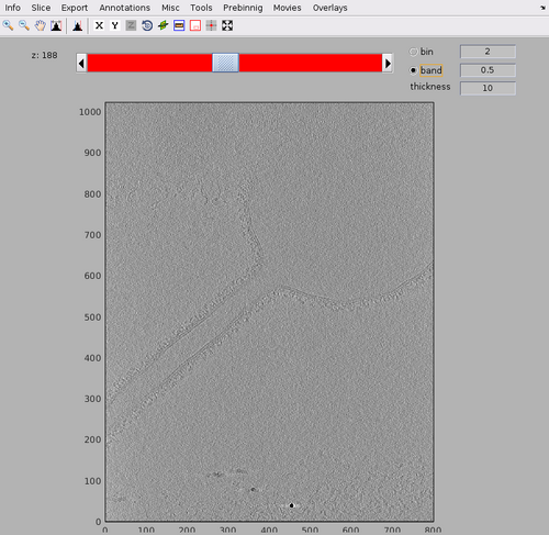
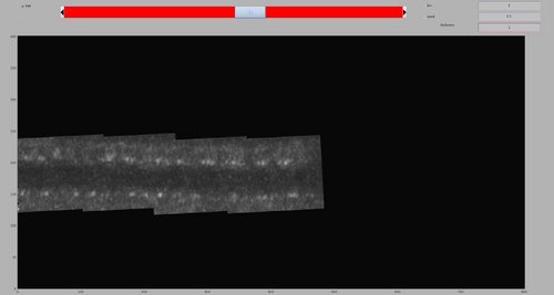
We can get a first glance on how the tomogram looks like:
dshow(tomofile);
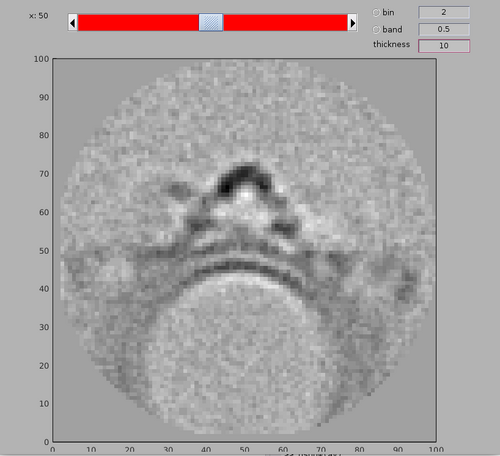
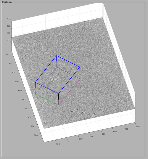
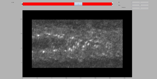
The tomogram should appear like the following figure. Note the tubulation starting from the liposome and the rich membrane coating. In this walkthrough, we are interested in highlighting the coating in the tubulation by template match.
Estimation of the missing wedge
We can quickly check the extent of the missing wedge in the tomogram. We extract a sample of the tomogram:
fragment = dynamo_read_subtomogram(tomofile, 'r',64,'c',[450,450,100]);
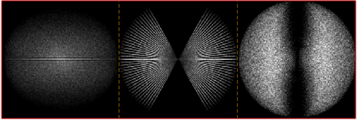
and plot a map of the distribution of the Fourier coefficients:
dynamo_wedge_estimate(fragment,'show',1);
The wedge estimation will show a nice symmetric tilt scheme from -60 to 60 degrees with 3 degrees steps.
Inspecting the template and model
In this walkthrough, a template and its mask are already provided. The template was generated by averaging ~50000 particles aligned with Dynamo.
The template can be loaded by:
av = dread('retromer_template.mrc');
And the mask can be loaded by:
mask = dread('retromer_mask.mrc');
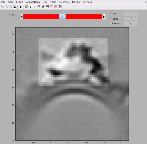
The template and mask positioning can be inspected with:
dshow(av+mask);
Note the central arc structure on top of the membrane bilayer of the tubulations. The mask contains the central arc as well as a small part of the membrane, but excludes the neighbouring arcs.
We can generate and write a low-passed version of the template with:
avbp = dynamo_bandpass(av,[3,10]);
dwrite(avbp,'retromer_template_filtered.mrc');
The two versions of the template can be compared with:
dtmshow({av,avbp});
Finally, a filament model [link] representing the tubulation is also provided. It can be loaded by:
mn = dread('mfilamentWithTorsion.omd');
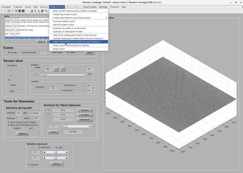
It can be inspected in the dtmslice GUI by first loading the tomogram:
dtmslice(tomofile);
And then selection the option "Import external file as model into pool (memory)" from the Model pool option.
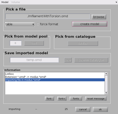
This will open a GUI allowing for the import of different model file. In this case type the model file name ./mfilamentWithTorsion.omd in the Pick a file option and click "create model" and then "ok"
This will draw the model in the dtmslice GUI. The model is meant to represent the rough backbone of the tubulation.
Generating a tesselation
There are multiple way to generate a tesselation policy for TM in Dynamo. Tesselation can be encoded either as a table or a specific dStar container. The function dpktomo.match.modelling.setUpTilingTable can be used to encode all the tesselation informations in a single dStar object. Each chunk can have the following fields:
- index: id of the chunk.
- tdrot, tilt and narot: the euler angles encoding the orientation of the template around which the TM scanning is done.
- posX, posY and posZ: the potion of the centre of the chunk in the coordinates of the tomogram.
- sizeX, sizeY and sizeZ: the side length of the chunk.
- cone_range or cr: orientations will be looked for inside a cone of this range around tdrot, tilt and narot.
- cone_sampling or cs: determines the scanning density inside the angular cone.
- inplane_range or ir or azimuthRange: in plane rotational range around narot.
- inplane_sampling or is: determines the scanning density for in plane rotations.
Additionally, a tesselation can be visualized using the function dpktomo.match.modelling.plotTesselation. The three main ways to create a tesselation are:
Automatic tesselation
Dynamo provides some function to automatically guess a tesselation policy from Dynamo models. Currently, Dynamo supports this functionality for Filament models, Membrane model and Dipole models.
The three main function are:
dpktomo.match.modelling.estimateTesselationForFilament
dpktomo.match.modelling.estimateTesselationForMembrane
dpktomo.match.modelling.estimateTesselationForDipole
Semi-automatic tesselation
As the geometric arrangement of may be complex, the automatic tesselation policy are designed to be conservative. However, this means that it is possible that a small intervention by the user would allow for better tesselations. A typical situation would be to use an automatic tesselation policy but with reduced volume. A function designed to help this process is dpktomo.match.modelling.setChunkSizes that suggest possible chunk sizes reductions.
Manual tesselation
Finally, a tesselation can be generated manually through the GUI or other means. The function dpktomo.match.modelling.setUpTilingTable can be used to assign specific chunk positions, orientations, sizes, angular ranges and angualar samplings to each element as required.
Automatic tesselation
In this walkthrough we will start with an automated tesselation policy generated by the filament model used to describe the tubulation position and orientation. First, the filament model must be used to generate a set of point describing the tubulation. This can be done in the same way as the creation of cropping points.
mn.radius = 35;
mn.subunits_dz = 12;
mn.updateCrop;
Lets set the default size of chunks to 300 and generate an automatic tesselation:
default_chunk_size = 300;
[chunkingTableLp,bigConeLp,chunkSizeLp] = dpktomo.match.modelling.estimateTesselationForFilament(mn,size(av),'chunkSize',default_chunk_size);
The information can be encoded in a dStar file using:
autoTesselationStar = dpktomo.match.modelling.setUpTilingTable(chunkingTableLp,'sizeX',chunkSizeLp,'sizeY',chunkSizeLp,'sizeZ',chunkSizeLp);
The tesselation can be quickly inspected by running:
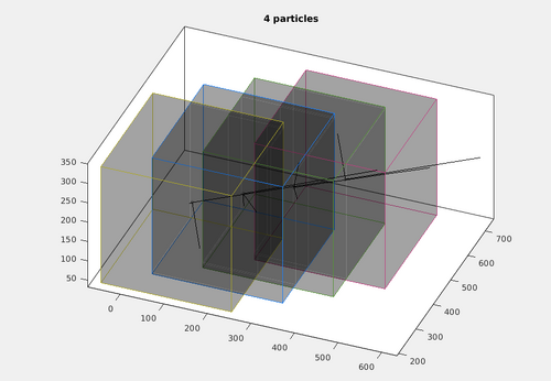
dpktomo.match.modelling.plotTesselation(autoTesselationStar,default_chunk_size,'alpha',0.2);
It can be noted that this tesselation includes four chunks oriented along the filament model.
Modifying an automatic tesselation
It can be noted in the previous image that the chunks overlap. This is expected because the borders of the chunks up to half of the size of the template will have a poorly defined cross-correlation and will be removed. In this case however, the automatic tesselation size is excessive. To allow for a more rapid computation, we can modify the automatic tesselation by forcing a reduction of the chunk sizes. dpktomo.match.modelling.plotTesselation is a convenient tool for rapid prototyping the chunk size. For example use:
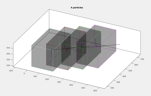
dpktomo.match.modelling.plotTesselation(autoTesselationStar,[180,300,180],'alpha',0.2);
By forcing the chunk to a non-cubic size, the dimensions of the tesselation chunks can be reduced while still tesselating the area of interest of the tubulation.
Manual tessellation
Tessellations can be created, loaded, modified and saved using the GUI functionalities.
These utilities are described in their own specific tutorial.
Running a model-aware TM
Preparing the template and the mask
As seen in the previous sections, the tesselation policy that will be used means that the template will be used to compute its cross-correlation scores with each chunk at each of its set of orientation. The set of orientations are defined by a cone oriented in the direction of the tubulation. However, this means that the template should be prepared so that its Z axis will correspond to the direction of the tubulation. Currently, the template Z axis is roughly corresponding to the normal vector of the tubulation membrane. As such, both the mask and the template should be recentered and reoriented:
avCentered = dynamo_normalize_roi(dynamo_shift_rot(avbp,-[0,3,0],[],[],0));
mCentered = double(dynamo_shift_rot(mask,-[0,3,0])>0);%mask is binarized
avCenteredRot = dynamo_rot(avCentered,[-90,90,-90]);
mCenteredRot = dynamo_rot(mCentered,[-90,90,-90]);
The new template and its masking can be inspected by:
dshow(avCenteredRot+mCenteredRot);
Running the project
At this point, we will use the new template and mask with the tesselation to do a TM computation restricted in angles and spaces. This means that we can afford to work without binning and with fine angular sampling.
tmBinning = 0;
angleSampling = 5;
The project can be named and run with:
nameTMproject = ['filt_r1gpu_bin_',num2str(tmBinning),'_cone60_slope_step',num2str(angleSampling)];


pts_R = dynamo_match(tomofile,avCenteredRot,'mask',mCenteredRot,'outputFolder',nameTMproject,'ytilt',[-60,60],...
'cr',60,'cs',angleSampling,'ir',360,'is',angleSampling,'bin',tmBinning,'gpus',1,'chunkSize',[180,300,180],'gpuByKernel',true,'matlabWorkers',10,'tilingTable',chunkingTableLp,'fineAssembly',1);
Note the flag 'fineAssembly'. This flag is used to request that the assembly of the cross-correlation chunks be done taking into account chunk overlap. AS in this cases overlap is present, the flag should be set to true.
The general syntax of the dynamo_match command and its main inputs is described in the basic TM tutorial. In summary, TM will be run on a tessellation with four chunk with sizes [180,300,180] with pre-orientation along the tubulation and a restricted cone of 60 degrees but full azimuthal range, both sampled each 5 degrees. The computation is requested to run on a single GPU, cpp accelerated rotations and finally assembled taking into account overlap.
This command required ~460 seconds of GPU computing time using a single NVIDIA GeForce RTX 4090.
Once the computations are finished, a folder with the project name and terminating with .TM will have been generated.
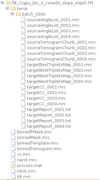
The project contain the assembled tomogram, cross-correlation map, the angular maps and a subfolder containing the specific results for each chunk in the tessellation.
Some common functionalities are the loading of a existing TM project with:
pts_check = dread('filt_r1gpu_bin_0_cone60_slope_step5.TM/process.mat');
The assembled tomogram and cross-correlation map can be inspected with:
 pts_check.showBinnedTomogram
 pts_check.showCC
Manipulating the cross correlation map
The results produced by the TM project can be manipulated using common Dynamo function. In this example, we well remove the signal from the gold bead from the cross-correlation map before extracting particles. Some useful representation tools are presented.
First, get the computed CC map. The TM project object can be used to get the file easily:
cc = dread(pts_R.io.getTargetBinnedCC);
And write it in the folder as reference:
dwrite(cc,[nameTMproject,'.TM/cc_original.mrc']);
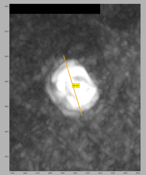
You may see that there is an area with high cross-correlation scores that have been caused by the presence of a gold bead. You can determine the position and size of the problematic area by using the functionalities of the dshow GUI:
dshow(cc);
We can create a cleaned version of the CC map by setting the values in the measured area to 0.
ccClean = cc;
ccClean(200-25:200+25,480-25:480+25,140-25:140+25) = 0;
The CC map in the project can be updated simply by:
dwrite(ccClean,pts_R.io.getTargetBinnedCC);
You can check that the update was successful by running:
pts_R.showCC
Advanced inspection of cross-correlation
At this time, the project is ready for particle extraction. However, it can be noted that the cross-correaltion map seems to present an interesting pattern that would give informations on the coating architecture. As such, in this section will introduce some way to highlight this with Dynamo functions. Firsly, it can be noted that the tubulation is oblique to the axes of the tomogram. The first action is to rotated the cross-correlation map with the command dtrot.
cc2 = drot(ccClean,[40,0,0]);
cc3 = drot(cc2,[90,-3,-90]);
ADJIUGIDIOAREMEBRER ANGLES CONVENTIONS
The result can be inspected by:
dshow(cc3);
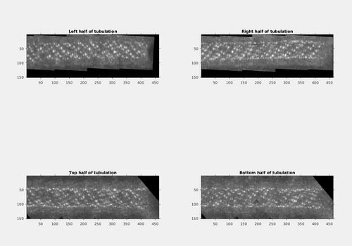
It would be nice to have a projection of only half of the tubulation at a time, so that the signal would be clearer. This can be done by generating four sub-volumes, each containing only half of the tubulation (top,bottom,left and right respectively), and the doing a maximum intensity projection. The identification of the limits of the sub-volumes can be done manually using the dshow GUI. In practice, the following projections can be generated:
ccmaxLeft = max(cc3(38:500,1:567,120:270),[],2);
ccmaxRight = max(cc3(38:500,568:end,120:270),[],2);
ccmaxBottom = max(cc3(38:500,500:650,80:175),[],3);
ccmaxTop = max(cc3(38:500,500:650,176:271),[],3);
And they can then by plotted:
figure;
subplot(2,2,1);
imshow(mat2gray(squeeze(ccmaxLeft)')); h1 = gca; h1.Visible = 'On';
h1.Title.String = 'Left half of tubulation';
subplot(2,2,2);
imshow(mat2gray(squeeze(ccmaxRight)')); h2 = gca; h2.Visible = 'On';
h2.Title.String = 'Right half of tubulation';
subplot(2,2,3);
imshow(mat2gray(squeeze(ccmaxTop)')); h3 = gca; h3.Visible = 'On';
h3.Title.String = 'Top half of tubulation';
subplot(2,2,4)
imshow(mat2gray(squeeze(ccmaxBottom)')); h4 = gca; h4.Visible = 'On';
h4.Title.String = 'Bottom half of tubulation';
The cross-correlation pattern along the tubulation is much easier to represent now.
The previous images suggest that a representation of the cross-correlation in cylindrical co-ordinates may be beneficial. However, to do this, the volume would need to be recentered and made such that the tubulation is collinear with the Z axis of the tomogram. First, a cubic area should be extracted:
volToInspect = cc3(10:409,368:767,1:400);
and it can be shifted and rotated in a single step with the command:
volToInspect = dynamo_shift_rot(volToInspect,[-10,-7,18],[90,90,-90]);
At this points, the limits of the cylindrical space to represent should be define. In this case, the full length of the tube will be represented for a radius of 10 pixels to 60 pixels and presenting the full 360 degrees of angular space sampled each 2 degrees.
Z = 1:size(volToInspect,3);
radius = 10:1:60;
angles = 0:2:360;
The cylindrical transformation can then by done with the provided volume2cylindercoordinates function:
[newvol] = volume2cylindercoordinates(volToInspect,angles,radius);
The new vloume can be inspected with dshow as usual, but maximum intensity projections are clearer.
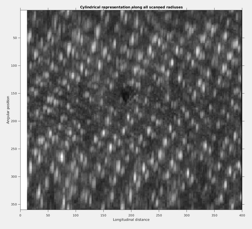
To inspect the cylindrical representation along all scanned radiuses do:
newvolmax1 = max(newvol,[],1);
I1 = mat2gray(squeeze(newvolmax1));
RI1 = imref2d(size(I1));
RI1.XWorldLimits = [0 Z(end)];
RI1.YWorldLimits = [angles(1) angles(end)];
figure;
imshow(I1,RI1);
xlabel('Longitudinal distance');
ylabel('Angular position');
title('Cylindrical representation along all scanned radiuses');
axis on;
To inspect the cylindrical representation along all scanned angles do:
newvolmax2 = max(newvol,[],2);
I2 = mat2gray(squeeze(newvolmax2));
RI2 = imref2d(size(I2));
RI2.XWorldLimits = [0 Z(end)];
RI2.YWorldLimits = [radius(1) radius(end)];
figure;
imshow(I2,RI2);
xlabel('Longitudinal distance');
ylabel('Radial position');
title('Cylindrical representation along all scanned angles');
axis on;
To inspect the cylindrical representation along all longitudinal positions do:
newvolmax3 = max(newvol,[],3);
I3 = mat2gray(squeeze(newvolmax3));
RI3 = imref2d(size(I3));
RI3.XWorldLimits = [angles(1) angles(end)];
RI3.YWorldLimits = [radius(1) radius(end)];
figure;
imshow(I3,RI3);
xlabel('Angular position');
ylabel('Radial position');
title('Cylindrical representation along all longitudinal positions');
axis on;
It can be noted that the tubulation was still not perfectly straight. However, even with this effect, the patter of the coating architecture presenting pairs of arcs in a general helical assembly is made evident.
Extracting the particles
At this point, the cross-correlation map can be used to find the positions and orientations of arcs.
n = 200;
myTableArc = pts_R.peaks.computeTable('npeaks',n);
This command can take a couple of minute to complete. This is because the template mask is used after each particle extraction to precisely ensure no particle duplicate are extracted even in crowded environment such as in this case. The actual particles can then be extracted with the usual Dynamo commands:
dtcrop(tomofile,myTableArc,'figure_1_fcrops_bin0a5',100,'mw',10);
The particle extracted will be of size 100x100x100 while the template was of size 64x64x64. This is a deliberate choice to allow for the inspection of the result even a long distances form the area of the template. The average can be assembled:
oa_figure_1_fcrops_bin0a5 = daverage('figure_1_fcrops_bin0a5','t','figure_1_fcrops_bin0a5/crop.tbl','mw',10);
To compare the average with the original template we need to remember that the template had been rotated. Both the average and the table can be rotated with:
T = dynamo_rigid('eulers',[-90,90,-90]);
Tinv = dynamo_rigid_inverse(T);
transformedmyTableArc = dynamo_rigid_apply(myTableArc,Tinv);
transformedAverage = dynamo_rigid_apply(oa_figure_1_fcrops_bin0a5.average,Tinv);
The average can be compared with the template visually with:
dshow('retromer_template.mrc');
dshow(transformedAverage);
The table can be inspected with:
figure
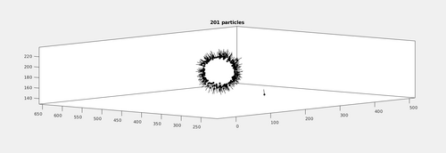
dtplot(transformedmyTableArc,'pf','oriented_positions');axis equal;
Additionally, a neighborhood analysis can be computed using that table.
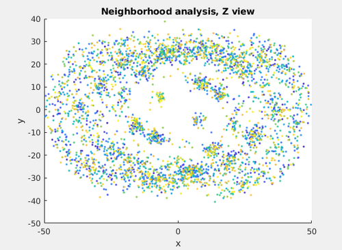
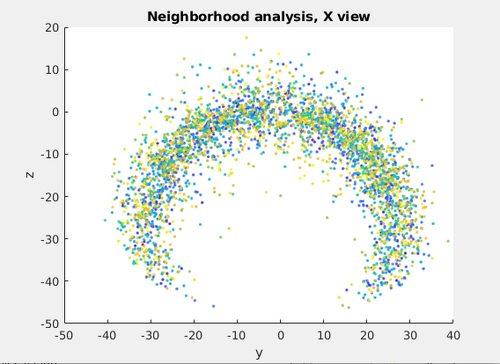
Neigh_transformedmyTableArc = dpktbl.neighborhood.analize(transformedmyTableArc,'distance',50,'modelColumn',13);
It can be inspected using the dtview with:
dtview(Neigh_transformedmyTableArc.coupleTable);
Even with a small set of 200 particles, the neighborhood analysis tries to highlight the local architecture of the coating. However, data from more tomograms would be required for a robust neighborhood analysis.
Additional functionalities
There are some additionally functionalities introduced with the model-aware template matching that can be useful even beyond the context of models and tesselations. Here the functionality of single chunk modus and on-the-fly reconstructions are introduced. An example of using oblique chunk is also shown.
Oblique chunks
In this section oblique chunks functionalities will be introduced. These functionalities are available from the GUI and allow for the creation of chunks of any orientation in a tomogram. This can be used to more finely limit the area and orientation with which TM can be executed. In this practical case, a single oblique chunk will be used to run a model-aware TM process on the entire length of the tubulation in a single shot.
Creating an oblique chunk
First, open the GUI with the tomogram data:
dtmslice('tomogram100_sm.mrc');
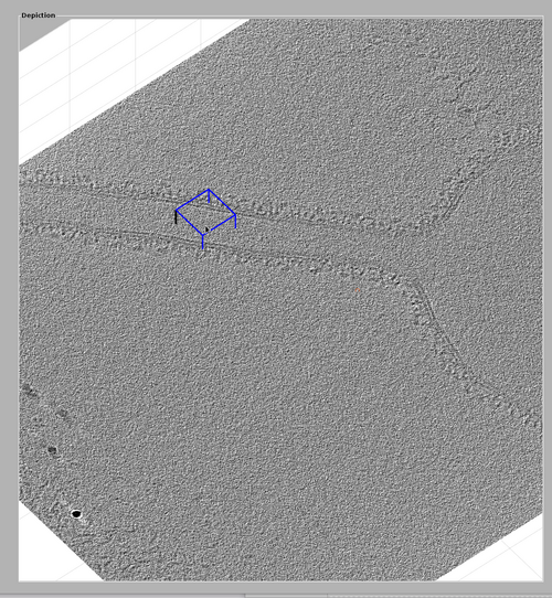
The goal is to create an oblique chunk in the GUI that contains most of the tubulation. An optimal chunk should follow the direction of the tubulation while being wide enough to contains the full coat and extra margins of at least the half-size of the template. To do this the basic functionalities of chunk manipulations are needed. These are: creating a chunk, resizing a chunk, moving a chunk and rotating a chunk. These utilities are described in more depth in their own specific tutorial.
Create a chunk by pointing the cursor on the tomogram and pressing the "B" key.
Resize a chunk by clicking an edge and dragging it with the cursor.
Move a chunk by shift-clicking an edge and dragging it with the cursor.
Rotate a chunk by alt-clicking an edge and dragging it with the cursor. This can also be done by right-clicking the chunk and then selection the option Change chunk orientation (into an oblique view). This will spawn a interactable lever that can rotate the chunk in any direction.
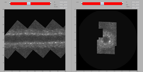
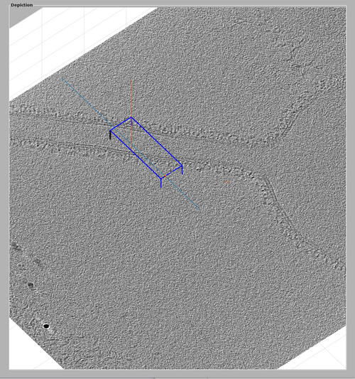
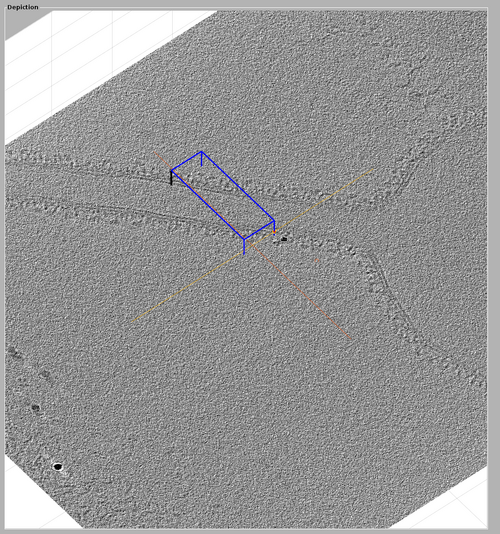
These basic operators should be used to create a chunk similar to the one shown in the next figure. A suggestion would be to: create the chunk, then increase its size and move it to contain the tubulation, then rotate it to the direction of the tubule with alt-clicking and finally reducing the size of the chunk.
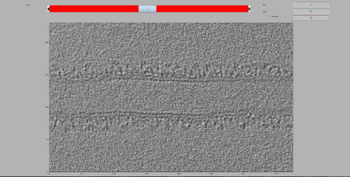
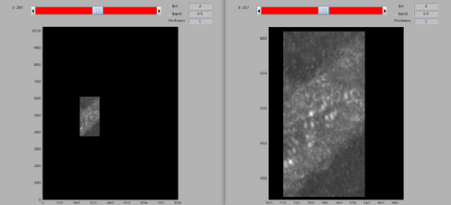
The volume included in the chunk can be inspected by right-clicking the chunk and selecting "show chunk (in tomoshow)". The volume should look similar to the one presented in the following figure.
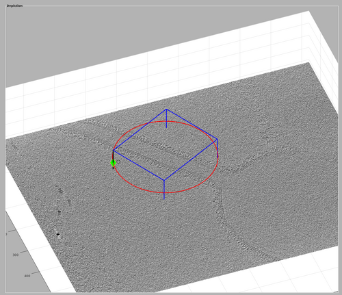
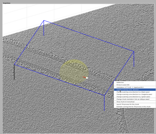
Finally, the chunk cone orientation should be defined. Right-click the chunk and select "change scanning cone direction". This will spawn a lever representing the direction of the scanning cone. Drag the lever to the direction of the tubulation like in the following figure.
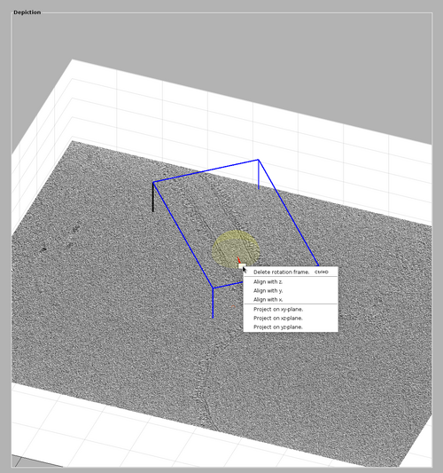
Once you are satisfied with the cone orientation, right-click the lever and select "delete rotation frame".
At this point a single oblique chunk has been defined as well as it cone orientation. This model can be saved by clinking the "save chunk distribution" option in the "Template Matching" tab at the top of the GUI. A model can be reloaded in the GUI by clicking the "load chunk distribution from .omd file"
Oblique TM
Once a chunk exists in the GUI, a localized TM process can be run on it. This is different from a normal model-aware TM in that it is run on a single chunk even if oblique and is run directly from the GUI.
Currently, the options to run TM projects embedded in the GUI require template, masks and missing wedge mask as files. As such, they need to be saved into disk. The template and mask can be saved with:
dwrite(avCenteredRot,'avCenteredRot.mrc');
dwrite(mCenteredRot,'mCenteredRot.mrc');
The Fourier mask encoding the missing wedged can be created and saved with:
fmask = dynamo_fmask(size(mCenteredRot),'range',[-60,60]);
dwrite(fmask,'fmask.mrc');
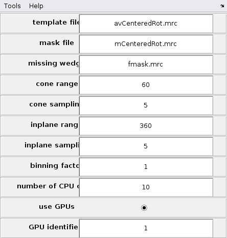
Now the TM parameters can be set in the GUI. This can be done by opening the Parameters GUI by selecting the "Template Matching" option on the top bar of the GUI and clicking "Settings for template match process". Update the fields template file, mask file and missing wedge with avCenteredRot.mrc, mCenteredRot.mrc and fmask.mrc respectively. Set the scanning ranges cone range and inplane range to 60 and 360 respectively. Set both cone sampling and inplane sampling to 5. This corresponds to similar TM parameters as the previous sections. Set the binning factor to either 0 or 1. A binning factor of 1 will speed-up the computations at the cost of cross-correlation maps of lesser quality.
Finally, set the computing parameters by selection the use GPUs button and setting number of CPUs to 10 and GPU identifier to 1.
The filled GUI should look like the one presented in the next figure.
At this point a TM project can be run on the oblique chunk. Right-click the chunk and select "Launch TM process for this chunk". This will automatically create a folder called "chunkTM.CTM" containing the oblique chunk and its resulting TM process. This computation will take a couple of minutes to compute if binning factor was 0 or less than one minute if binning factor is 1.
The results of the oblique TM can be accessed from "chunkTM.CTM/process.TM". For example, the resulting cross-correlation map can be inspected with:
dshow('chunkTM.CTM/process.TM/cc.mrc');
The usual post-processing functionalities of a TM process remain available as well.
Single chunk modus
Single chunk modus is a strategy for computational speed-up exploiting a different parallelization strategy. By default, the TM algorithm in Dynamo will parallelize computations by assigning each chunk to a different GPU or MATLAB worker if in CPU modus. However, some projects may require to instead have fine angular scanning in a restricted spacial region. In those cases, it is more natural to work with a single chunk and parallelize in the angular space instead. This can be done in Dynamo using the single chunk modus.
A computation example will be done using the data from the prevois sections. This example will be done in GPU modus using only one GPU. This choice was made to allow for the experiment to be tested with limited hardware, but the natural approach would be to have as many GPU as selected parallelization items (this can be done by giving the GPU as an array, for example 'gpus',[1,2,3,4]).
Set up a similar project as before, but with a angular cone amplitude of 180 degrees and only on the third chunk:
nameTMprojectSC = ['filt_r1gpuSC_bin_',num2str(tmBinning),'_cone60_slope_step',num2str(angleSampling)];
singleChunkTile = chunkingTableLp(3,:);
tmBinning = 0;
angleSampling = 5;

pts_RSC = dynamo_match(tomofile,avCenteredRot,'mask',mCenteredRot,'outputFolder',nameTMprojectSC,'ytilt',[-60,60],...
'cr',180,'cs',angleSampling,'ir',360,'is',angleSampling,'bin',tmBinning,'gpus',1,'chunkSize',...[180,300,180],'gpuByKernel',true,'matlabWorkers',10,'tilingTable',singleChunkTile,'fineAssembly',1','singleChunkModusFlag',1,'singleChunkModusNumberOfSplits',4);
By setting the flag singleChunkModusFlag to true and forcing singleChunkModusNumberOfSplits to four, TM will use single chunk modus to parallelize the computation of the selected chunk by splitting the scanned angles into four groups and then assembling the resulting cross-correlation maps using fineAssembly.
The resulting CC map can be inspected with:
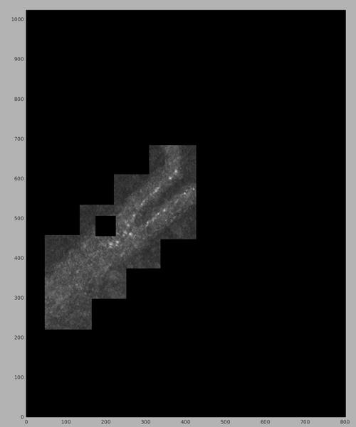
pts_RSC.showCC;
Note the presence of only the selected chunk. It can be noted by comparing with the previous results that the shape of the CC map in the chunk is similar to the previous one, even though this time an angular cone with 180 degrees of aperture was used.
This can be highlighted by inspecting the resulting cross-correlation maps that were computed. Load the parts of the CC map:
chunkPart1 = dread([nameTMprojectSC,'.TM/temp/batch_0000/targetCC_0001.mrc']);
chunkPart2 = dread([nameTMprojectSC,'.TM/temp/batch_0000/targetCC_0002.mrc']);
chunkPart3 = dread([nameTMprojectSC,'.TM/temp/batch_0000/targetCC_0003.mrc']);
chunkPart4 = dread([nameTMprojectSC,'.TM/temp/batch_0000/targetCC_0004.mrc']);
And lets inspect the all using the dmapview GUI:
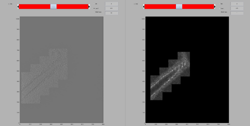
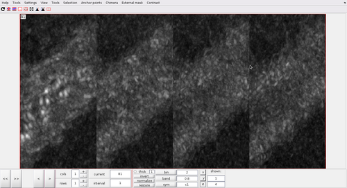
dmapview({chunkPart1,chunkPart2,chunkPart3,chunkPart4});
Note how the first chunk is the one that looks more structured and dominates during the assembly of the final CC map. This is because it was the part that scanned the set of angles closest to the tesselation chunk vector, and a such included the set of angles more probable to be correct. It can be noted that the exact set on angles using in each computation can be loaded for example with:
chunkPart1scannedAngles = dread([nameTMprojectSC,'.TM/temp/batch_0000/sourceAngleList_0001.mrc']);
On-the-fly chunk reconstruction
Finally, it is possible to run TM in Dynamo with an input aligned TS instead of a tomogram. In this case, each chunk will be reconstructed on-the-fly from the tilt series instead. All other functionalities of the TM module in Dynamo can be used with on-the-fly chunk reconstruction too. However, more informations must be given to the process to compute properly. An example of on-the-fly TM syntax is provided.
Let say that two different tomograms of different dimensions and centers have been generated from the same single tilt series TS.mrc using:
ts = dread('TS.mrc');
ts_filt = dpktomo.rec.applyRampFilter(ts);
outputBPbasic = dpktilt.math.backproject([479,463,200],ts_filt,tiltAngles,'mw',10);
outputBP = dpktilt.math.backproject([531,320,200],ts_filt,tiltAngles,'mw',10,'shiftTomogramCenter',[32,64,11]);
As tomogram may have different shapes, TM will need two additional information beyond the tilt series file and its set of angles:
-tomogramCenter: used to define the coordinates of the tomogram on which chunking tables are defined.
-stackSize: used to define the implicit tomogram of a tilt series. The X and Y components are the dimention of a micrograph in the tilt series, while the Z component is the wished tomogram thickness.
Basic on-the-fly reconstruction TM:
pts_GPUkernel = dynamo_match('TS.mrc',TEMPLATE,'mask',TEMPLATE_MASK,...
    'outputFolder','onthefly_GPUkernel',...
    'ytilt',[-60,60],'cr',360,'cs',30,'bin',0,'mw',10,'gpus',1,'gpuByKernel',true,...
    'assembleLive',1,'sc',160,'angles',tiltAngles,'tomogramCenter',outputBPbasic.stack3DCenter,'stackSize',([(outputBPbasic.stackSize(1:2)),200]));
Model-aware on-the-fly reconstruction TM with tesselation defined on a tomogram of different dimensions that the tilt series:
pts_GPUkernelCh = dynamo_match('TS.mrc',TEMPLATE,'mask',TEMPLATE_MASK,...
    'outputFolder','onthefly_GPUkernelCh',...
    'ytilt',[-60,60],'cr',360,'cs',30,'bin',1,'mw',10,'gpus',1,'gpuByKernel',true,...
    'assembleLive',1,'fineAssembly',1,'sc',80,'angles',tiltAngles,'tomogramCenter',outputBP.stack3DCenter,'stackSize',([(outputBPbasic.stackSize(1:2)),200]),'tilingTable',tilingTable);
