Walkthrough on hexagonal lattice coherence through neighborhood analysis

Neighborhood analysis

Neighbourhood analysis stands at the forefront of methods used to investigate geometrical lattice parameters and offers a wide spectrum of visualization tools. This technique is precise, targeting specific elements, yet broad enough to facilitate overarching interpretive analysis. At its core, the method constructs a latent space of connections by mapping the relative positions of neighbouring particles onto a reference framework. This mapping involves a reorientation process, wherein the 'N' closest neighbours are repositioned within the reference particle's coordinate system, adjusted for its orientation. The richness of the latent space—characterized by the number and nature of these repositioned features—is dictated by a defined distance threshold. This threshold ranges from a minimal couple, representing the closest inter-particle distance, to the maximal extent, linking every particle within the neighbourhood to the reference point.

For additional insights into neighborhood analysis, visit this page.

Data

We will use data from the initial gold standard alignment derived from five tomograms of immature HIV-1 virus-like particles.

Downloading

The data can be downloaded from this google drive.

Inspecting data

First, open a new local terminal and navigate to the directory containing the tutorial dataset and project.

Let's inspect the contents:

>> dfile template.em
   
   filetype: volume
   
   size: 192 x 192 x 192 

>> dfile table.tbl
 
   filetype: table
   
   size: 7068  x 35, aligns: 7068, averages: 7068 

These files represent an average as a template and its associated metadata (i.e., table). We will focus on the table data.

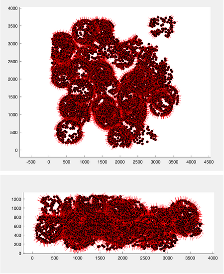
To visualize the particles along with their normals:

tbl = dread('table.tbl');
figure;
h = dpktbl.plots.sketch(tbl,'haxis',gca());
h.zlength.value=100;

VLPs particle positions and normals.

Prepare (meta)data

Let's select a couple of Virus-Like Particles (VLPs):

tblT2V2 = tbl(tbl(:,20) == 2 & tbl(:,22) == 2, :);
tblT2V5 = tbl(tbl(:,20) == 2 & tbl(:,22) == 5, :);
tblT2V3 = tbl(tbl(:,20) == 2 & tbl(:,22) == 3, :);

To visualize:

figure;

subplot(1, 3, 1);
dpktbl.plots.sketch(tblT2V5);
title('Ideal');
pbaspect([1 1 1]);

subplot(1, 3, 2);
dpktbl.plots.sketch(tblT2V2); 
title('Slightly flat surface');
pbaspect([1 1 1]); 

subplot(1, 3, 3);
dpktbl.plots.sketch(tblT2V3); 
title('1/4 missing, flat top');
pbaspect([1 1 1]); 

Selected VLPs. From left to right: ideal, medium, and low quality instances.

Indeed, we will analyze three different VLP quality instances.

Get mean distance to closest neighbor

To find the optimal distance threshold, we will use the following function to calculate the mean distance to the closest neighbor:

function [meanDst, stdDsts] = mean_distance_to_closest_neighbor(pts);
numPts = size(pts, 1);
minDsts = zeros(numPts, 1);

for i = 1:numPts
   dsts = pdist2(pts(i,:), pts);
   dsts(i) = Inf;
   minDsts(i) = min(dsts);
end

meanDst = mean(minDsts);
stdDsts = std(minDsts);
fprintf('Mean distance: %.4f\nStandard deviation: %.4f \n', meanDst, stdDsts);
end

Invoke the function like so:

[meanDst, stdDsts] =   mean_distance_to_closest_neighbor(tbl(:,24:26)+tbl(:,4:6));

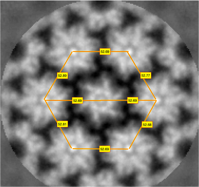
The mean distance to the closest neighbor is around 50-60 pixels.

Mean distance: 50.42
Standard deviation: 12.23

For a sanity check, you might also measure the lattice directly on the average volume:

dshow template.em

Overplot average and hexagonal lattice measurements.

Neighborhood analysis computation

Here, we conduct the neighborhood analysis with a distance threshold set as the mean distance plus the standard deviation:

tblT2V3N = dpktbl.neighborhood.analize(tblT2V3,'distance',meanDst+stdDsts,'modelColumn',22);
tblT2V2N = dpktbl.neighborhood.analize(tblT2V2,'distance',meanDst+stdDsts,'modelColumn',22);
tblT2V5N = dpktbl.neighborhood.analize(tblT2V5,'distance',meanDst+stdDsts,'modelColumn',22);

Then, we will need the couple table since it is our new representation (i.e., latent space):

tblT2V3NC = real(tblT2V3N.coupleTable);
tblT2V2NC = real(tblT2V2N.coupleTable);
tblT2V5NC = real(tblT2V5N.coupleTable);

Now, let's visualize first-order distance clusters with synchronized viewing:

datasets = {tblT2V3NC, tblT2V2NC, tblT2V5NC};
titles = {"Incomplete + flat surface", "Slightly flat surface", "Ideal"};

fig = figure;
ax = gobjects(1, length(datasets));

for i = 1:length(datasets)
   ax(i) = subplot(1, length(datasets), i, 'Parent', fig);
   pcshow(datasets{i}(:, 24:26), 'Parent', ax(i));
   pbaspect(ax(i), [1 1 1]);
   % Set titles using text, since the title function was not working
   xl = xlim(ax(i));
   yl = ylim(ax(i));
   zl = zlim(ax(i));
   titlePos = [mean(xl), yl(2), zl(2)];
   text(ax(i), titlePos(1), titlePos(2), titlePos(3), titles{i}, ...
       'HorizontalAlignment', 'center', 'Color', 'white', ...
       'FontSize', 14, 'FontWeight', 'bold', 'BackgroundColor', 'black');
end

link = linkprop(ax, {'CameraUpVector', 'CameraPosition', 'CameraTarget', 'CameraViewAngle', 'XLim', 'YLim', 'ZLim'});
setappdata(gcf, 'StoreTheLink', link);

for a = ax
   rotate3d(a, 'on');
end

First-order distance clusters obtained vía neighborhood analysis. From left to right: low, medium, and high quality instances.

The color, by default, represents the Z-axis. Notice that the better the quality of the VLP, the less sparse each cluster is.

Local analysis - lattice coherence

To quantify lattice coherence, we apply k-means clustering and calculate the Euclidean norms for each centroid. The standard deviation of these norms provides a measure of cluster sparsity and hence, lattice coherence.

We encapsulate this process in a function:

function [idx, cc_final, results, results_std] = perform_lattice_analysis(data, symm)
   [idx, cc_final] = kmeans(data, symm);
   results = vecnorm(cc_final, 2, 2); 
   results_std = std(results); 
end

Then, execute the analysis:

symm = 6; 
[idx_ideal, cc_ideal_final, results_ideal, std_ideal] = perform_lattice_analysis(tblT2V5NC(:,24:26),symm);
[idx_slightly_flat, cc_sf_final, results_sf, std_sf] = perform_lattice_analysis(tblT2V2NC(:,24:26),symm);
[idx_incomplete_and_flat, cc_implt_final, results_implt, std_implt] = perform_lattice_analysis(tblT2V3NC(:,24:26),symm);

Display results neatly in a table

resultsTable = table(std_ideal, std_sf, std_implt, 'VariableNames', {'Ideal', 'SlightlyFlat', 'IncompleteFlat'}, 'RowNames', {'StandardDeviation'});

disp(resultsTable);

This will output:

                              Ideal             SlightlyFlat        IncompleteFlat                       
                        __________________    _________________    _________________
                          
   Standard deviation    0.0933777687916592    0.321031652546273    0.574732108201886

As demonstrated, the qualitative degree of imperfection correlates with our lattice coherence measurements.