HIV1 workshop
Contents
- 1 Goal of the walktrough
- 2 Structure of the walktrough
- 3 Recovery of acquisition parameters
- 4 Motion correction and dose weighting
- 5 CTF estimation and correction
- 6 Alignment and reconstruction
- 7 Dynamo models and particles
- 8 Subtomogram averaging
- 9 Fourier shell correlation
- 10 RELION conversion
- 11 Final RELION refinement
Goal of the walktrough
This walktrough was designed to describe and discuss the steps necessary to go from the raw microscope data of a cryo-electron tomography experiment to a high-resolution average with the relative particles position and orientations.
In practice the EMPIAR dataset entry 10164 (https://www.ebi.ac.uk/empiar/EMPIAR-10164/) is used to analyse the structure of the GAG coat of immature HIV1 virus-like particles.
A set of common cryoem software tools will be used such as: MotionCor2, CTFFIND 4, IMOD, Dynamo, Chimera, RELION and Bsoft.
One of the goals is to show how these different softwares can be used in a synergistic approach to recover high resolution data. Additionally, the step-by-step description of the workflow is meant to allow users to be able to achieve the final result even by using other similar softwares that were not introduced in this walktrough.

Structure of the walktrough
The full HIV1 walktrough pipeline has been split into multiple sequential steps. Each of these steps corresponds to a subsection of this wiki page. It is possible to reach an average with about ~4 A of resolution starting from 5 tilt series by following all of the steps described in this walktrough. The process to create a tilt series from the microscope movies is only mentioned and discussed in the "Motion correction and dose weighting" subsection.
However, depending on the hardware available, a full execution of this pipeline can easily take a week of computing time. Additionally, the generated data consumes considerable amounts of memory resources. As such, this walktrough is has been constructed to be scalable. The full version of the walktrough code package is divided into two sections: scripts and data. The following figure represents the package tree. The data part includes all of the pre-computed intermediate files.
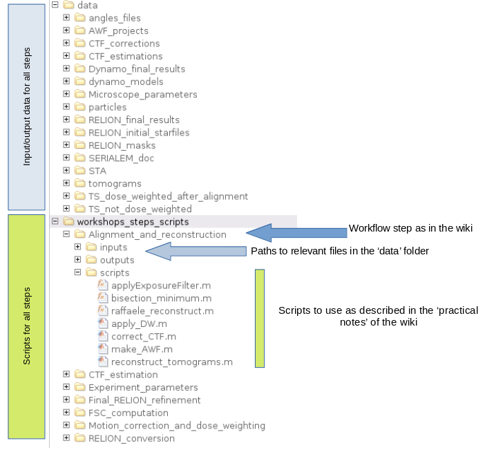
There are two main approaches on the implementation of walktrough with different scales of memory and computing resource requirements: with pre-computations or full execution. The two approaches are described in the following tables.
| with pre-computations |
|---|
| Requires an already filled 'data' section. |
| Does not require large computing resources. |
| Intended for in-person workshop. |
| The 'data' section has been made available from a physical memory. |
| The 'script' section can be downloaded from https://drive.google.com/file/d/16POOrfRc6Vw_XSidNWhcGvQzvbjivuN-/view?usp=drive_link. |
| The script generally do not need modification. |
| By default most scripts process only one tilt series. This is done to save computing time. |
| The scripts access their inputs data from the 'data' section. |
| full execution |
|---|
| Does not require an already filled 'data' section. |
| Requires large computing resources. |
| Intended for individual practical use. |
| The 'data' section starts has mostly empty. The 'data' section can be downloaded from https://drive.google.com/file/d/1k4bLLswsacYdIGcNRc76YcbAiycxyPuX/view?usp=drive_link. |
| The 'script' section can be downloaded from https://drive.google.com/file/d/16POOrfRc6Vw_XSidNWhcGvQzvbjivuN-/view?usp=drive_link. |
| The scripts will need modifications. |
| The scripts need to be modified to process all of the tilt series. The scripts are already structured to simplify the needed modifications. |
| The scripts access their inputs data from the 'data' section. As such, the 'data' section needs to be filled with the outputs of the scripts after each step. |
As mentioned previously, the "full-execution" approach requires some limited script modifications. The matlab scripts have been generally structured so as to present three parts. The first part consists of the paths to the input and output files. The second part is the section of parameters. The third part is a for loop on the input tilt series. As such, the typical modifications necessary for the "full-execution" approach are limited to the first part, ensuring that the inputs for all five tilt series are given.
Additionally, in the "full-execution" approach, the results of the scripts are used to populate the empty 'data' section so that the following scripts may be able to access their input files. This means that the files need to be positioned in the correct folder tree location and with a consistent file name. To help with this process, each step has an output text file in its folder with the path and file names that need to be applied to ensure consistency.
Recovery of acquisition parameters
A number of important characteristics of a cryo-electron microscopy experiment are necessary to properly process the data.
As such, this first step of the walkthrough is a guided process to recover the relevant information for this datasets.
In general, other that the sample movies themselves, the required information can be split in two parts: the characteristics of the microscope and the characteristics of the experiment.
The needed microscope characteristics are:
- voltage.
- spherical aberration.
- amplitude contrast.
- gain reference.
The needed experiment characteristics are:
- pixel size.
- image size of the tilt series.
- dose.
- tilt scheme.
The walkthrough is based on the EMPIAR dataset entry 10164. The corresponding paper is: Florian K. M. Schur et al., An atomic model of HIV-1 capsid-SP1 reveals structures regulating assembly and maturation.Science353,506-508(2016). DOI:10.1126/science.aaf9620. and the EMD deposition is EMD-4015, https://www.ebi.ac.uk/emdb/EMD-4015?tab=experiment.
The microscope parameters are describe in the paper. The microscope that was used is a FEI TITAN KRIOS with an acceleration voltage of 300 kV. The nominal spherical aberration is of 2.7 mm. The amplitude contrast in cryo-electron tomography is ~10%. In the following the value of 7% is picked.
The gain reference is not available for this experiment. However, the gain reference is only useful during motion correction of the movie. In this walkthrough we will start with already motion corrected and stacked tilt series. As such, the gain reference is not required for this walkthrough. In any case, more information on motion correction and on the gain reference is provided in the next section.
The experiment characteristics still need to be found. Firstly:
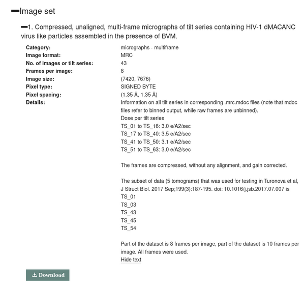
access the EMPIAR dataset entry 10164 by accessing the link https://www.ebi.ac.uk/empiar/EMPIAR-10164/
Go to the "Image set" section of the EMPIAR page.
The subset of tilt series that will be used in the walktrough are TS_01, TS_03, TS_43, TS_45 and TS_54.
The dataset in the EMPIAR consists in movies. As such, the Frames per image of 8 means that each movie is a set of 8 frames. In addition, we can note that Image size is (7420,7676). This refers to the size of a movie. In summary, if one of the movies in this EMPIAR dataset would be stored as a matrix, it would have the shape 7420x7676x8.
The pixel size can be found by inspecting Pixel spacing, which get a pixel size of 1.35 A, and in the Details section the information of the dose can be found.
Note the dose and pixel size of the tilt series TS_01, TS_03, TS_43, TS_45 and TS_54.
The size of the image size of the tilt series can now be found.
Update the variable root to the path the the data folder.
Then run:
dynamo_read_mrc_size([root,'data/TS_not_dose_weighted/01.mrc'])
This will return the dimensions of the tilt series TS_01. The order is size in x, size in y and size in z. In a tilt series the z dimension is the tilt. Now run:
dynamo_read_mrc_size([root,'data/TS_not_dose_weighted/43.mrc'])
You will note that the tilt series TS_01 is one tilt shorter than the tilt series TS_43. By inspecting the tilt angles files:
open([root,'data/angles_files/43.rawtlt'])
open([root,'data/angles_files/01.rawtlt'])
you can see what tilt angle is has been removed in the tilt series TS_01. Additionally you can:
Annotate the image size of the tilt series.
You can note that the x and y sizes of the tilt series are half of the size of the movies that was indicated in the EMPIAR
Image size section. This is because during motion correction the micrographs are cropped to avoid aliasing. More information on this can be found in the paper: Electron counting and beam-induced motion correction enable near-atomic-resolution single-particle cryo-EM, Li, Xueming, Mooney, Paul, et al. Nature Methods, 2013, https://doi.org/10.1038/nmeth.2472
The final experiment characteristic needed is the tilt scheme. This information is generally already known, but it can also be recovered from the microscope SerialEM logs. These logs are provided for this dataset in the EMPIAR, but only partially: the logs refer to a binned output and do not present information on the dose. This is why the dose information was presented in the Details section instead.
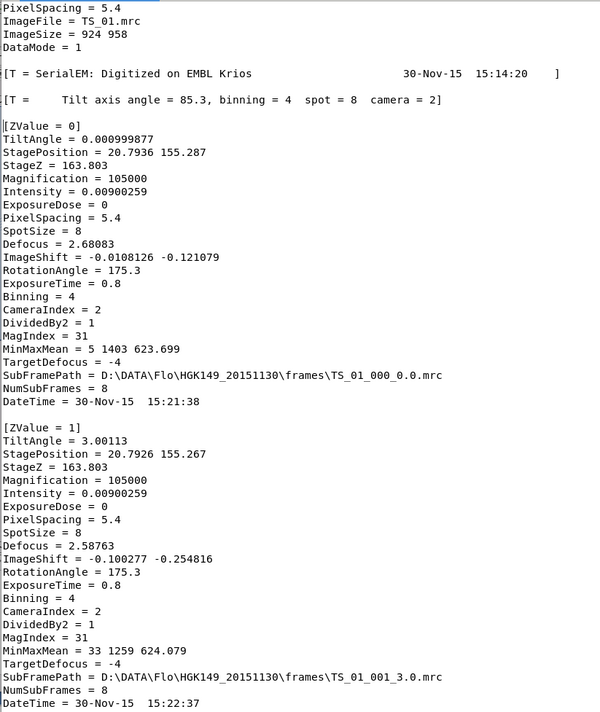
One of the these serialEM logs has been made available in the data folder. You can open it:
open([root,'data/SERIALEM_doc/TS_01.mrc.mdoc'])
The log file starts with an header of six lines with some general characteristics. The binned SerialEM pixel size is consistent with eh pixel size noted in the EMPIAR.
Note the Tilt axis angle
The tilt axis angle in SerialEM is meant to be the angle between the axis of rotation of the sample during tilting and the axis of the detector.
The log file is then split in section by the line [ZValue=????]. This line separates the different microscope acquisitions (i.e. each movie generation). The number of ZValue indicates the order of the acquisitions. Taking the screen shot as an example: the first block is about the first movie taken because the Zvalue is 0. The tilt angle was 0, that is the first acquisition was take with a flat sample. The second block is about the second movie because the Zvalue is 1. The second tilt angle was +3.
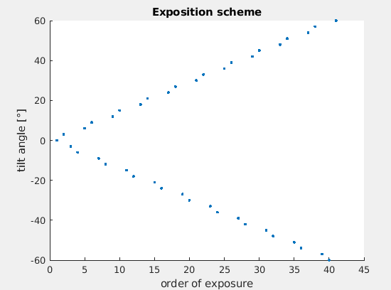
This means that by inspection the log the tilt scheme can be recovered. The custom function parse_metadata will do this task. Run:
[tiltAngles, indices] = parse_metadata([root,'data/SERIALEM_doc/TS_01.mrc.mdoc']);
And you can inspect the acquisition scheme by running:
figure;
scatter(indices,tiltAngles,'.');
xlabel('order of exposure');
ylabel('tilt angle');
title('Exposition scheme');
We can note that the tilt scheme is a dose-symmetric with steps of 3 degrees like: 0,+3,-3,-6,+6,+9,-9,...
A copy of the tilt scheme in an appropriate format for the following steps is already computed and can be inspected by:
n_of_preexposures = csvread([root,'data/Microscope_parameters/order_list.csv']);
Motion correction and dose weighting
Initial comments
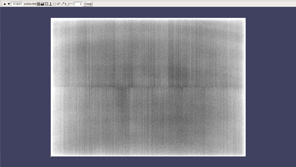
The output of a microscope after a tilt series acquisition will be a gain image and a movie for each tilt. In practice, often a single gain file is used for all the tilt series experiments done in a microscope session. The following figure present an example of a gain reference file from a different dataset.
Some more information on reference gains can be found at the link:
https://zmb.dozuki.com/Guide/TEM+-+TFS+Titan+Krios+G3i+-+2a:+Collect+Gain+References+for+the+K3/183
The first steps that can be done are the correction of the sample motions caused by the electron beam exposure and the dose weighting.
In this case, MotionCor2 will be used (https://emcore.ucsf.edu/ucsf-software).
MotionCor2 will use the movies and the gain to generate a motion-corrected micrograph per each movie. MotionCor2 should not be used to do the dose weighting at the same time as the motion correction. This is because the implementation of the dose weighting procedure in Motioncorr2 has been deigned for single particle experiments, not cryo-electron tomography.
Dose weighting is meant to generate a more strict filtering of high-frequency components of the power spectra in frames that have been exposed to large doses of electrons per square angstroms. This means that the order of exposition of the tilts is crucial. This process will be done in this walktrough after the alignment step.
Some steps in the following walktrough are more adapted to either the dose weighted micrographs or the not dose weighted micrographs, so it is often good to keep both available.
Finally, the micrographs should be stacked in order of tilt (generally from negative angles to positive angles).
Input
- a set of microscope movies.
- a gain.
- microscope parameters: pixel size, voltage, spherical aberration and amplitude contrast. (SPECIFY)
- the tilt angle of each movie.
- the order of tilt exposition.
Practical notes
Here is an example of a MotionCor2 call that will generate both a dose weighted and a not dose weighted micrograph:
'motioncorr2 -InMrc movie.mrc -OutMrc tilt.mrc -Patch [5 5] -Iter 30 -bft 200 -Tol 0.5 -Kv 300 -PixSize 2.73 -FmDose FMDOSE -InitDose INITDOSE -FtBin 1'
where INITDOSE will depend on the number of previous tilts in the exposition scheme. As mentioned before, the dose weighting results of Motioncorr2 are meant to be used in single particle experiments. As such, in this case, the dose weighting will instead be done during the tilt series alignment step using a Matlab script.
Note that the previous motioncorr2 call did not use a gain. If you want to use the gain you can add it with the -GAIN PATHTOGAIN flag. Sometimes the gain needs to be flipped or rotated depending on what where the setting of SerialEM during the acquisition and this can be done with the -RotGain and -FlipGain flags.
More practically, dynamo has a set of common preprocessing scripts that can be downloaded at: https://github.com/C-CINA/TomographyTools/tree/master/matlab_files
With a particular note on the script preprocessing_script.m, motioncor2Wrapper.m and applyExposureFilter.m.
The script applyExposureFilter.m can be used to apply dose weighting on a micrograph that was already motion-corrected.
Outputs
- the dose weighted tilt series.
- the not dose weighted tilt series.
CTF estimation and correction
Initial comments
The CTF of each micrograph can be estimated and corrected in different ways. In this case, ctffind4 (https://grigoriefflab.umassmed.edu/ctffind4) was used to estimate the CTF parameters and IMOD was used to correct it using the ctfphaseflip function of IMOD (https://bio3d.colorado.edu/imod/doc/man/ctfphaseflip.html).
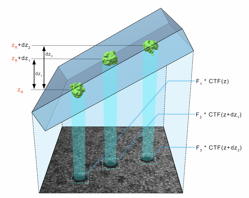
CTF can be tricky in cryoem because of the low dose per micrograph and the fact that the sample is tilted, causing the CTF to be different in different regions of the micrograph. In addition, the thickness of the sample means that even the CTF estimated in a region of the micrograph is in actuality caused by the entire thickness of the sample.
These problems can apply both to the CTF estimation and the CTF correction. Some strategies that can be used to limit these problems are going to be presented in the following.
CTF estimation: It can be noted that the CTF can be done either on the dose weighted or on the not dose weighted tilt series. It should be more proper to use the not dose weighted micrographs, but in practice using the dose weighted micrographs can be more straightforward. In our case, ctffind4 was used on the not dose weighted tilt series.
CTF correction: ctfphaseflip locally corrects the CTF (that was estimated over the entire micrograph) by correcting the local defocus in each area using the geometric Z-offset generated by the tilt. However, this means that ctfphaseflip requires an aligned tilt series. Indeed, the automatic fiducial-based tilt series aligner of dynamo can be used to correct the CTF after generating the aligned tilt series (see following steps).
Input
for the CTF estimation:
- the not dose weighted tilt series.
for the CTF correction:
- the aligned, dose-weighted tilt series.
- the CTF parameters of the tilt series.
- the tilt angles.
- the microscope parameters.
Practical notes
At this time CTF estimation part will be executed. The CTF correction will be done during the alignment and reconstruction step.
The relevant information will be found in the 'CTF_estimation' folder.
The script use_CTFFIND4_to_estimate_CTF.m will use ctffind4Wrapper.m to estimate the CTF parameters using CTFFIND4.
Note that this is done by making a system call for the CTFFIND4 software. As such, it is necessary to know where the software has been installed.
Line 178 of ctffind4Wrapper.m should be changed to be able to reach the CTFFIND4 executable. An easy way to check if the executable can be reached is to try which ctffind4 in the terminal.
Update the variable root to the path the the data folder.
Find thye ctffind4 installation:
which ctffind4
Once you have the path to the ctffind4 installation you can update the script.
change line 179 of ctffind4Wrapper from:

    fprintf(fileID,'ctffind4 <<EOF\n');    % path to ctffind4 installation (adapt if necessary)

to:

    fprintf(fileID,'PATHTOMYCTFFIND4EXECUTABLE <<EOF\n');

where PATHTOMYCTFFIND4EXECUTABLE was just identified.
Now the CTF microscope parameters need to be given to the script.
Update the script use_CTFFIND4_to_estimate_CTF.m in the parameters section.
Now the script can be run:
run use_CTFFIND4_to_estimate_CTF.m
CTFFIND4 will generate three files for each tilt series: a 'XXX_diag.mrc' file, a 'XXX_diag.txt' file and a 'XXX_diag_avrot.txt' file. Some notes on the role these files:
- 'XXX_diag.mrc': this file will present visually the estimated CTF on the power spectra of each tilt. The dynamo command dshow can be convenient to quickly inspect the results
- 'XXX_diag.txt': this file will annotate the CTF parameters estimated for each tilt.
Finally, the CTFFIND4 result are converted in a '.defocus' file compatible with IMOD. This is done because IMOD will be used later to correct the CTF. This conversion is done in use_CTFFIND4_to_estimate_CTF.m by calling the function ctffind2imod.m
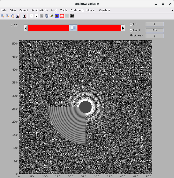
Inspect a CTFFIND4 result with dshow:
dshow('01_diag.mrc')
You will get something like this figure:
The Z dimension scroller correspond to moving between different tilts, and correspondingly to different relative sample thickness as well as accumulated doses.
The parameters found by CTFFIND4 can be inspected by opening the XXX_diag.txt file:
open('01_diag.txt')
Outputs
for the CTF estimation:
- CTF parameters of the tilt series.
for the CTF correction:
- the aligned, dose-weighted, CTF-corrected tilt series.
Alignment and reconstruction
Initial comments
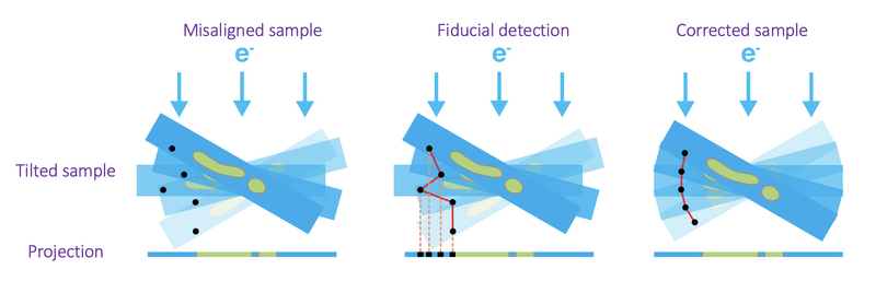
Each tilt series needs to be aligned to then be able to reconstruct them in tomograms. In this approach a fiducial-based automatic alignment is used. The general concept of fiducial-based alignment is shown in the following figure. In particular, the alignment procedure will describe the alignment as a general rotation angle for the entire tilt series and then additional shifts in x and y directions for each tilt. Generally, the rotation angle can be seen as the angular difference between the axes of the detector and the axis of rotation of the sample. The x and y shifts try to model the imprecision in the sample movement during each tilt acquisition.
Once the tilt series has been aligned, the ctfphaseflip correction can be applied as described in the previous section.
Finally, the aligned, dose-weighted, CTF-corrected tilt series can be used to reconstruct the tomograms. Weighted backprojection is the preferred method to generate the tomograms that will be used to generate subtomograms for the STA. SIRT can be used to generate tomograms with better contrast to more easily annotate the data with dynamo models.
The automatic fiducial-based workflow (AWF) in dynamo can be used to do: the alignment, the estimation of CTF parameter, the CTF correction and finally the tomogram reconstruction. The AWF can be used either through the GUI or programmatically.
From the dynamo wiki:
https://www.dynamo-em.org/w/index.php?title=Walkthrough_on_GUI_based_tilt_series_alignment
https://www.dynamo-em.org/w/index.php?title=Walkthrough_on_command_line_based_tilt_series_alignment
The AWF will generate an AWF folder in which the results will be saved.
https://www.dynamo-em.org/w/index.php?title=Tilt_series_alignment_workflow_folder
The quality of an alignment is difficult to measure, but some general considerations can be made:
https://www.dynamo-em.org/w/index.php?title=Considerations_for_tilt_series_alignment_in_IMOD
In this practical setup, a script will be used to automatically and programmatically align all tilt series, but the CTF handling and the reconstruction will be done separately. This choice was made to present in mode detail how to achieve a CTF correction and to mention how other softwares (like IMOD) can be used to reconstruct TS that were aligned using dynamo.
Input
- (not dose-weighted) tilt series.
- gold beads parameters.
- CTF parameters.
Practical notes
The relevant information will be found in the 'Alignment_and_reconstruction' folder.
The work will be split in four parts: the alignment, the dose weighting, the CTF correction and finally the reconstruction.
cd to the folder workshops_steps_scripts/Alignment_and_reconstruction/scripts
Practical notes: alignment
The alignment will be generated using the script make_AWF.m. This script will programmatically initialize and run the dynamo automatic fiducial-based tilt series alignment but skipping the CTF handling and the reconstruction.
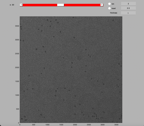
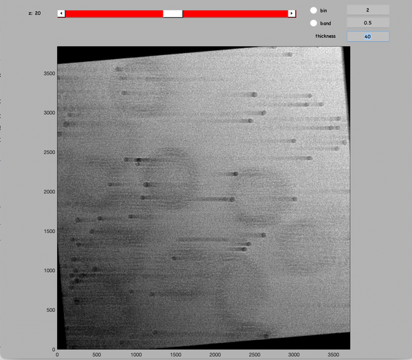
The algorithm only requires as parameters the gold bead radius, the gold bead mask, the template sidelength and the binning to apply. These parameters are determined by inspecting a tilt series. Open the first tilt series by running:
dshow([root,'data/TS_not_dose_weighted/01.mrc']);
This will open the dshow GUI representation of the tilt series.
Using the GUI tools:
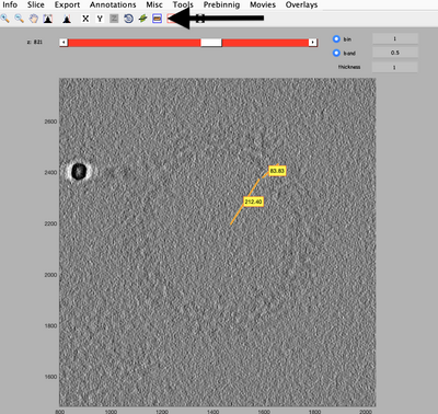
Use the GUI binning tool to render the gold beads easier to see
The binning applied is purely visual. The dimensions of the tilt series does not change and this means that the measurement with the distance tool are in full-scale pixels.
Use the measuring tool to estimate the radius of the gold beads
This procedure allows to estimate the radius of the gold bead and the binning to apply. This is because the AWF will initially detect the gold beads using template matching on the visually binned tilt series just as it was done manually now.
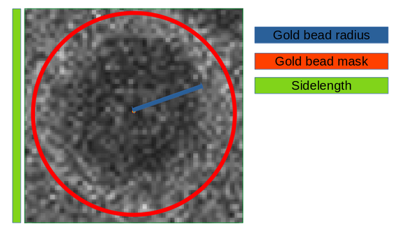
The next figure present visaully the relationship between parameters gold bead radius, the gold bead mask radius and the template sidelength.
Generally we suggest to set the mask radius parameter as about 50% bigger than the beads radius and then set the template sidelength as the smallest that can contain the mask diameter.
Use this rule of thumb to estimate the gold bead radius and sidelength parameters
The required data to set up an AWF are: the unaligned TS, the tilt angles, the pixel size and the gold bead parameters. In addition, the dimensions of the of the reconstructed tomogram are used in the AWF. However, in this case, these values will act as fill-ins because the actual reconstruction will be done separately.
Update the parameters of the script make_AWF.m (except zFullSize_a, as said before)
The script will do the alignment only for the first tilt series because of time limitations. Precomputed alignment are proveided in the data/AWF_projects folder.
Once the alignment as been completed, one (or all five if the for loop at line 33 has been changed to for 1:n_tomos) .AWF project will have been generated. In particular, the aligned tilt series can be found in '.AWF/align/alignedFullStack.mrc'. The actual alignment parameters can be found in the files 'stackAligner.dyn' and 'stackAligner.star'. The information in the two files is essentially the same, but in a human-readable format in the .star file and a dynamo-readable format in the .dyn file. Inspect the alignment parameter by running:
open('HIV_AWF_fortestsdata/TS_not_dose_weighted/01.AWF/align/stackAligner.star')
You will see the alignment parameters shift in x, shift in y and psis angular correction. Psis is the angle between the tilt axis of the sample and the axis of the camera.
compare the psis value found in the alignment with the SerialEM tilt axis angle
The difference of angle should be less than one degree. By default AWF scans the psis angle at intervals of 0.1 degrees. It is sometimes possible that there might be an offset of 180 degrees in the estimation of the tilt axis angle in different softwares depending on how the axis are defined.
The overall alignment can be inspected in multiple ways. First, to see the information about the markers found, run:
u.info.markers;
You should see in the log that there are no empty frames. The number of empty frames is the number of frames removed by the AWF and those frames will not appear in the aligned tilt series.
Then you can inspect the fitting log. Run:
u.info.fit;
You will see the same psi as in the one in stackAligner.star. The value of the rms is also provided.
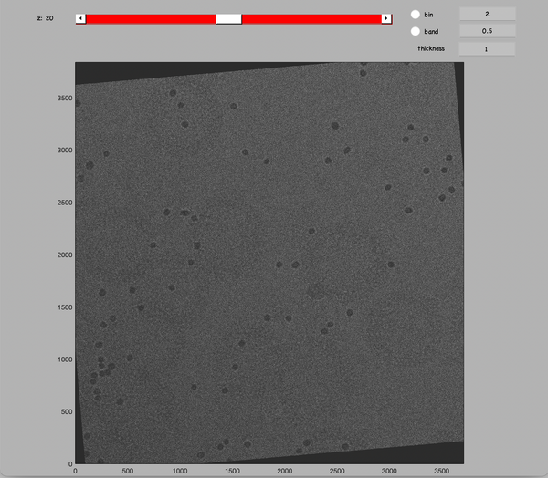
A visual inspection of the aligned tilt series can alos be done. Run:
u.view.stack.alignedFull();
The gold beads should appear like they are moving horizontally between tilt.
Increase the thickness value of the GUI to more than the number of tilt to have a superposition of all aligned micrographs
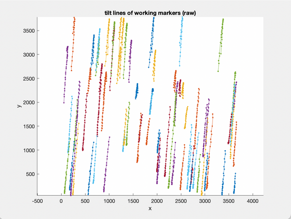
You can see the original tilt lines with:
u.view.tiltLines.unaligned;
It can be noted that in this tilt series the tilt lines are mostly vertical before alignment and horizontal after alignment.
Practical notes: dose weighting
The dose weighting will be done using the script apply_DW.m. This script will dose weight a TS by calling the function applyExposureFilter.m. This function implement a dose filtering based on the paper "Measuring the optimal exposure for single particle cryo-EM using a 2.6 Å reconstruction of rotavirus VP6", Grant & Grigorieff, elife 2015.
The required data to do the dose filtering are the aligned tilt series, the dose per tilt and the tilt scheme. The tilt scheme information has been provided as a .csv file and merely notes the order of exposition of all tilts.
Update the parameters of the script apply_DW.m
The apply_DW.m script will generate .mrc files of dose weighted tilt series. Run the script:
run apply_DW.m
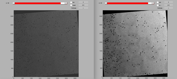
You can compare the tilt series before and after dose weighting by running:
dtmshow({'01_DW.mrc',[root,'data/AWF_projects/HIV_ali_AWF/TS_01/01.AWF/align/alignedFullStack.mrc']});
This will open two synchronized representation of the tilt series before and after dose weighting. The difference will be more obvious in tilt that have been subjected to larger accumulated doses.
Practical notes: CTF correction
The CTF correction will be done using the script correct_CTF.m. This script do a system call to the ctfphaseflip function of IMOD.
Update the line 24 of the script correct_CTF.m from:

    system(['ctfphaseflip -InputStack ',path_to_dwTS{tiltserie},...

to:

    system(['PATHTOYOURIMOD/ctfphaseflip -InputStack ',path_to_dwTS{tiltserie},...
a way to check that this worked is to type:
system(['PATHTOYOURIMOD/ctfphaseflip'])
if the path is correct you should get a description of the function inputs.
ctfphaseflip is much faster with a GPU. If you have one available you can simply add the -gpu 0 flag.
The required data to do the dose filtering are the aligned and dose-weighted tilt series, the tilt angles, the CTF parameters (in .defocus format) and the microscope parameters.
Update the parameters of the script correct_CTF.m
In general, it is possible that alignment procedure may have discarded some frames (for example, black frames). In this case, it is important to ensure that the tilt series .mrc file, the CTF .defocus and the angle file match.
The correct_CTF.m script will generate .mrc files of CTF-corrected tilt series. For time constrains, this is done only on the first tilt series. As usual, precomputed results can be found in the folder data/CTF_corrections.
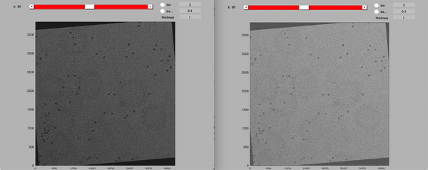
You can inspect the tilt series before and after CTF correction by typing:
dtmshow({'stackCTF_DW_ali_01.mrc',[root,'data/TS_dose_weighted_after_alignment/alignedFullStack_TS01_DW.mrc']});
An easy way to check if CTF correction was applied to inspect the black areas cause by the alignment. A CTF-corrected tilt series will present a wave pattern in these areas.
Practical notes: reconstruction
The reconstruction will be done using the script reconstruct_tomograms.m. This script will use the dynamo function that reconstructs a tomogram using the weighted back-projection approach. It is the same function that would have been used had we wanted to do the reconstruction directly in the AWF project.
The required data to do the reconstructions are the dose-weighted, CTF corrected aligned TS, the tilt angles and the requested Z thickness of the tomogram.
Update the parameters of the script reconstruct_tomograms.m with a thickness of 2000
The reconstruction is equivalent to an IMOD reconstruction using the tilt .... --ROTATE 90 command of a tilt series aligned with the IMOD-compatible alignment parameters. These alignment parameters were generated in the AWF folder as the files 'stackAlignerImod.dyn' and 'stackAlignerImod.star'.
Launch the reconstruction by running:
run reconstruct_tomograms.m
For time constrains, this is done only on the first tilt series. As usual, precomputed results can be found in the folder data/tomograms.
You can check the dimensions of the tomogram with:
dynamo_read_mrc_size(['recCTF_DW_ali_01.mrc'])
and you can inspect the tomogram with: dshow(['recCTF_DW_ali_01.mrc']).
However, this is a large full-scale tomogram, so it will take a long time to load. As such, it might be best to inspect only binned tomograms. This will be done in the next section.
Outputs
- tomograms
Dynamo models and particles
Initial comments
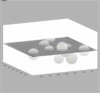
After the tomographic reconstruction, the user needs to identify the target of the biological investigation. In general, one would like to have a vectorial representation that captures the geometry of the particle distribution. This process is known as particle picking (sometimes referred to as volume annotation).
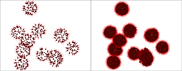
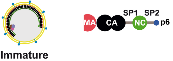
Here, the focus is on the main structural component of HIV-1: the polyprotein Gag. Since, for instance, its ordered cleavage causes a dramatic structural rearrangement of the virus to the mature, infectious virion. In the immature virus particle, Gag is radially arranged (left, figure below). The particle segmentation model capturing such a surface is reasonably spherical/ellipsoidal. Therefore, the choice should be a dipole. This Dynamo model class is very convenient since it allows the user on-screen interaction to be reduced in directly clicking the centers that roughly correspond to the presence of individual particles.
Once the dipole sets for the particle's global region are ready, we proceed with "seed oversampling". This technique involves creating cut points along the models to extract smaller sub-volumes. Understanding the underlying distribution, especially the degree of homogeneity and symmetry, is key to selecting a sensible oversampling configuration; it is key to success on the road to high resolution. Although, at this stage of the project the positions of these cropping points are not supposed to be realistically centered on a copy of the polyprotein of interest.
At the end of the extraction process, you should have a crop table, a set of particles, and a template (i.e. the average of the subvolumes).
Input
- tomograms
Practical notes
Prior to a more practical depiction, it is essential to pause and become aware of the data organisation and naming convention. In this regard, the user is advised to have a highly consistent data structure. The project is about to grow in size. Therefore, errors probably mean lots of hours of work lost.
For more information:
https://www.dynamo-em.org//w/index.php?title=Practical_Suggestions_for_Tomographic_Reconstruction
Preparation and management of data
The organization of folder can be created by running:
hiv1Dirs = {'catalogue', 'particles', 'projects'} ;
cellfun(@(x) mkdir(x), hiv1Dirs);
the data structure should look as
    .
    │
    └── workplace
       ├── catalogue
       ├── particles
       └── projects
Next, move the current directory to catalogue
cd catalogue
Then,
Create a '.vll' file inside the catalogue folder containing absolute paths to the tomograms (one path per line).
A '.doc' file that also contains the path (absolute or relative, it is recommended to use absolute paths) to the tomograms and their volume ID needs should also be stored in the catalogue folder. That is, exactly the same content as your '.vll' with an ID in the beginning of each tomogram path. Remember, in MATLAB, indexing start from 1.
Create a '.doc' file inside the catalogue folder containing and ID followed by the absolute paths to the tomograms (one ID and path per line).
The line
dcm -create c000 -fromvll tomograms.vll
will help to create a catalogue, as a centralised manager of tomograms.
The GUI will pop up as soon as the catalog 'c000.ctlg' is called via
dcm c000
Now,
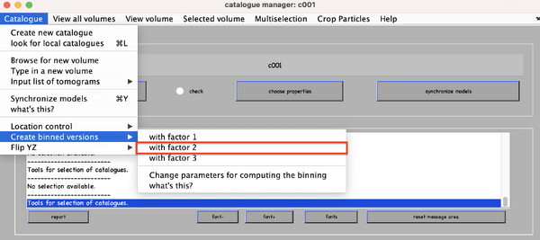
Create the binned version of the tomogram selecting a factor of 2.
Note, these versions will be saved inside the folder of the tomograms, not inside the catalogue folder.
Particle picking
As commented before, this part involves on-screen interaction. For this, the main tool to work is the dcm. Just make sure to be inside the right directory ('./catalogue’).
Then,
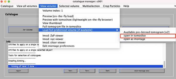
Open one tomogram through the catalogue in ''dtmslice'' (load the previously binned versions, else, there is risk of potential delay and slow performance).
The first thing one will probably want to do is to change the contrast, bandpass it and, if not binned, play with a certain thickness.
Adjust the tomogram appearance.
Next,
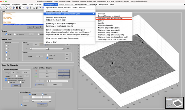
Interactively create a dipole model set.
To generate the surface parametrisation of the VLPs, every visible target is marked with only 2 clicks: one on its center and one on its surface (press keyboard letter '''c''' and '''n''', respectively). Pressing '''enter''' saves the current dipole in the set and activates the next dipole.
The annotation does not need to be very accurate at this point, since the following alignment projects are designed to cope with inaccuracies introduced at labelling (up to 40 pixels are tolerable). The VLP quality is not relevant, thus try to maximise the number of annotations (approx. 8 to 9 VLPs per tomogram). The reason is that bad/junk particles will be excluded in a dedicated step later on. Although, depending on your specific pipeline and requirements, data curation might be important and, for other projects, you might want to have only good quality targets. Especially if you have a lot of tomograms.
Just make sure to save the dipoles to disk after the labelling of each tomogram is done.
The catalogue will manage for you folder creation and naming (e.g., './c000/tomograms/volume_1/models/mdipoleSet.omd').
Repeat the annotation process for the remaining tomograms.
Particle extraction
As commented in the opening remarks, the challenge in this section is to set the oversampling configuration. You will need to define a distribution of boxes based on the expected distribution of physical particles. To this end, open one of the binned tomograms:
dtmshow -otf pathToTomogram
In order to get the support needed w.r.t. the decision making process:
Use the ruler tool to measure distance.
Decide the optimal relation of:
- physical distance between the particles / sampling distance in pixel of dipole model surfaces
- physical size of the particle / side length that you ask for the particle cropping.
Once you have decided the oversampling configuration, the time for scripting has come. Get out the catalogue directory to the workspace and:
mkdir scripts
Then, simply move or copy the downloaded wild card script and open it via
movefile([pathToDownloads '/Dynamo_models_and_particles/scripts_wc/model_workflow.m'], './scripts')
open model_workflow.m
Remember, you will find a [!!] and/or an NaN wherever scripts need to be completed.
Is time for to fill in the quantities missing to:
Configure geometry related inputs ( i.e., sampling distance and the box size for particle extraction ).
Add the separation of crop points onto the vesicle model.
Additionally, the following task will need to be completed
Create crop points on VLP surface (oversampling).
Add the radius to vesicle.
Create crop table from vesicle model.
Finally, each dipole on the annotated tomogram is processed by running the model_workflow.m script.
Thus,
run model_workflow.m
This will create a regular lattice of coordinates (about 800 to 1,000 per tomogram) on the surface. These coordinates will be the center of the extracted subvolumes. For each tomogram and the associated set of dipoles a regular lattice of cropped subvolumens, the output will be a crop table, and a template of the initial average of those oriented particles (subvolumes). Technically, the so-called particle extraction process involves the creation of a merged table with dynamo_table_merge. Then, the cropping of sub-volumes with dtcrop. It will not only crop the table but it will also manage the sub-volume tagging. Finally, templates generate averaging all the particles with daverage. While the user can implement its own version, the recommendation is to use the in-house version given that it accounts for missing wedge compensation.
For more details about particle extraction, Dynamo average, and Fourier compensation, the reader is referred to:
https://www.dynamo-em.org/w/index.php?title=Particle_extraction
https://www.dynamo-em.org//w/index.php?title=Daverage
https://www.dynamo-em.org/w/index.php?title=Fourier_compensation_during_averaging
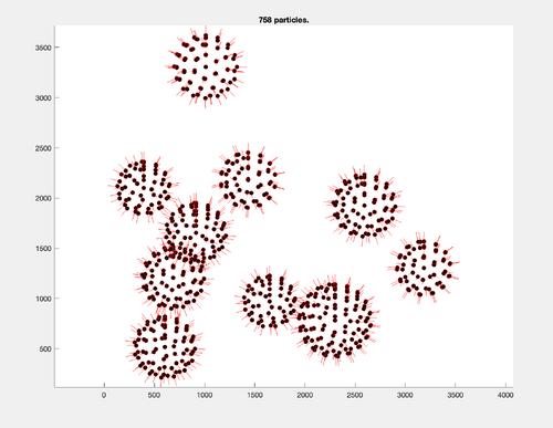
How to find out if everything went well? It is time to do a sanity check.
Display final table positions of the seed oversampling along with their orientations:
finalTable = dread([pathToTargetParticleFolder '/crop.tbl']);
figure; title([num2str(size(finalTable,1)) ' particles.']);
h = dpktbl.plots.sketch(finalTable,'haxis',gca());
h.zlength.value=100;
A simple average of the extracted particles, without alignment, should already reveal the VLP curvature of the surface. To check:
finalAverage = dread([pathToTargetParticleFolder '/template.em']);
dshow(finalAverage)
Outputs
- dipole models.
- initial cropping table.
- particles.
Subtomogram averaging
Initial comments
Once multiple copies of individual protein complexes are extracted from the tomograms, the next step is to mutually align and average these sub-volumes. The ultimate goal: to yield a signal-enhanced 3D structure up to sub-nanometer or even near-atomic resolution. This technique is known as subtomogram averaging (StA).
The general StA approach seeks to recover the common signal in the collected particles by an iterative process that alternates alignment and averaging steps. In simple words, aligning subtomograms is the process of computing for each available particle the set of shifts and angles that will bring them to a common reference. When all the particles have been aligned, they can be averaged together. This process will run in an iterative way in order to gradually improve the attained resolution. In practice, the full dataset is split into two independent datasets that are aligned and averaged separately. The half-sets are commonly referred to as even and odd and are divided based on the particle indexing number. The 2 half-maps are needed to validate the final map via gold standard Fourier shell correlation (FSC) computation.
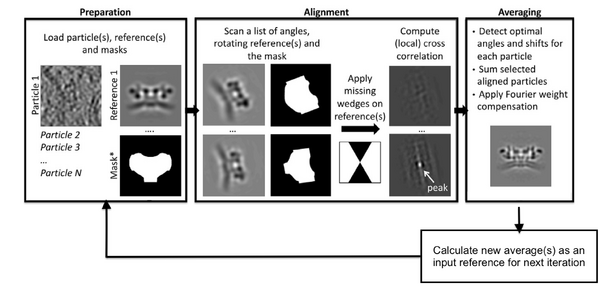
However, reaching a point where the quality is sufficient to opt for gold-standard refinement is neither simple nor straightforward. With Dynamo as the core tool for high-demand computation, and Chimera for interactive particle selection within the density maps, the protocol to be followed is as outlined here:
Creation of initial reference.
- Data preparation and management.
- Alignment project for references.
Extraction of first per tomogram average.
- Data preparation and management.
- Particles centering and re-averaging.
- Alignment project per tomogram.
Computing an average of averages.
- Data preparation and management.
- Alignment project for average of averages.
Extraction of second per tomogram average.
- Data preparation and management.
- Subboxing.
- Alignment project per tomogram.
Extraction of coarse half maps.
- Data preparation and management.
- Particle filtering, registration, and re-cropping.
- Gold standard alignment.
Extraction of refined half maps.
- Data preparation and management.
- Particle filtering and new initial reference computation.
- Gold standard alignment.
Input
- tomograms.
- initial cropping table.
Practical notes
If the reader is already familiar with dcp, they may choose to skip ahead to the next section.
The alignment project is one of the most important objects in Dynamo. It is used to design the operations carried on the particles, to select and configure the environment where the actual computations will occur, to start the computations and to access and visualise the results. For more information about the elements involved:
https://www.dynamo-em.org//w/index.php?title=Alignment_project
The command line–based workflow is convenient since allows for the projects to be streamlined and automatised for increased throughput. To create the project, it is enough to give its name (a string) to dcp.new (for instance, dcp.new(theNameOfMyProject)).
Regarding file management, it is ideal to work with folders for particle storage. In some cases, it will be sufficient to initialise the new project with this folder, the table, and the mask(s). This is not possible when more than one tomogram is used. Each set of particles will be inside a different folder. In this case, access is centralised by creating a '.star' file. In MATLAB, the user must store everything in generic containers (cell array). Create a dynamo object dpkdata.containers.ParticleListFile.mergeDataFolders, and use the writeFile to actually write the file to disk. Dynamo objects are versatile, and, for example, dcp, offers the flexibility to use the same functions with different file formats.
Once all the files are ready, these can be linked to the existing project through dvput followed by the name of the project, the flag, and the element (for example, dvput(theNameOfMyProject, 'data', theFolderOfMydata) or dvput(theNameOfMyProject, 'data', starFileName)). Just make sure to create default masks in case you have not created ones ad hoc for your target, dvput(theNameOfMyProject, 'masks', default).
The user can choose to work fully interactively. If so, the GUI dcp is the main tool. The Wizard will open unless the flag show is passed to 0 at creation time (e.g., dcp.new(theNameOfMyProject, 'show', 0)). It will indicate with a different color what should the user input onto the project.
Analogous to the CLI version, if applicable, do not forget to click the option for default masks use.
Note, that in contrast to other softwares, the data (particles) and metadata (table(s)) are explicitly different files. Therefore, at this stage of the project, it is highly recommended for the user to get acquainted with table convention that can be found here:
https://www.dynamo-em.org/w/index.php?title=Table_column_convention
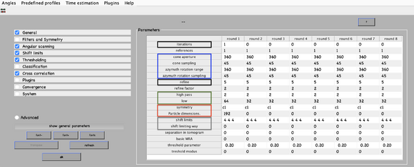
Next, numerical parameters will be configured. They define the mathematical part of the project. Among others, in terms of sets of angles to scan, shifts to allow, used bandpass, angular refinement policy or binning options. It might feel overwhelming at first. Expertise about each parameter of such configuration is required to select the optimal configuration in one-shot.
A good start for analysis is the direction of the proteins based on the particle model ( defined by the vertical axis first two Euler angles). For instance, if you know the proteins are more or less orthogonal to the membrane, there is no point in scanning 360 degrees. On the other hand, the sampling of the cone must be coupled to the status of the project. That is to say, in an initial state, when there is uncertainty about the orientation, it makes no sense to sample every degree. However, a good estimate could be every 10 degrees. This reasoning also applies if you have reached your subvolumes by template matching, since at most, you have a directional error of 30 degrees.
As rule of thumb, the third Euler angle (defining the inplane rotation) can be assumed to be biased. Either for the missing wedge, or for some arbitrary sampling of the particles. Therefore, azimuth angle randomization shall be performed. The function needed is dynamo_table_randomize_azimuth. Do not forget to create a template with the new table, daverage, and save to disk, dwrite . Again, depending on your target, a global scanning might be necessary. In contrast, if you have some premise that 90 degrees is sufficient, as is the case for HVI-1, go ahead and set it up.
For those users who are still not confident with the orientation parameters (depicted in blue in the figure of numerical parameters), the recommendation is to complete the advance starters guide. In this walkthrough, the orientation is unravelled into separate projects. The links to the tutorial and data are as follows:
https://www.dynamo-em.org/w/index.php?title=Advanced_starters_guide
https://wiki.dynamo.biozentrum.unibas.ch/w/doc/data/fhv/crop.rec
To configure the position parameters, think about how likely are the particles to be shifted in x,y, and z. In most cases, after a couple of trials cropping, more precision can be expected in x,y. Whereas the z, is known to be harder to fit. Thus, it seems reasonable to permit more translational freedom in that direction. The modus of this area of search, unless having a good reason, should be set to 1. Meaning that the limits are understood as the center of the particle. Note that mode 0 is dangerous, and accumulated shifts can lead to very large displacements. These two values are squared in gray in the figure.
Regarding filtering, try to be realistic. The default value for high pass is okay. It will prevent noise from ruining the alignment. However, the low pass filter needs to be a meaningful value. In any case, even if you are not sure, do not push Nyquist. Instead, support this decision by visualising the binned template, for instance, you might use dshow and calculate the pixel size with dynamo_resolution . Although, if you have half maps available, it is worth it to compute the FSC curve.
Symmetrization is a powerful technique. However, it should initially be avoided since it can induce bias. As the project evolves, if the target happens to be clearly symmetric, exploit this fact. Just be aware that symmetries that are not a subset of the sampling scheme are not recommended. Namely, any other family but circular families (cn).
The quality, signal-to-noise ratio, and homogeneity of the target will determine the number of iterations needed. It is a trade-off between computational time and the improvement being obtained. To do this, you can open another instance of MATLAB and buy the results.
The logical trend is that with higher resolution, the parameters can be more restrictive, accompanied by a larger particle size, and the low pass filter cutoff frequency reduced. Generally, the higher the level of detail, the more iterations will be needed for convergence.
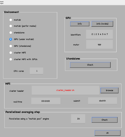
The computational environment will be determined by the resources you have available. Try to maximise the number of cores and GPUs as this is directly proportional to the computational time. If it is a long project, you probably do not want to use gpu 0. So that the pc used to visualise the results is not affected by the computations. In case you are sharing resources, make sure that there is no mismatch between the system ids and MATLAB (remember that the indexing for your system starts at 0 and for MATLAB at 1).
The project is now ready to be checked, unfolded, and launched. Do not worry if some path is broken or not found, dcp will warn and prevent the project's launching unless it can be done safely. For this, you might want to run:
outputCheck = dynamo_vpr_check(theNameOfMyProject);
if isempty(outputCheck)dvrun(theNameOfMyProject,'unfold',true);elsedisp('Project not safe.')end
Creation of initial reference
Place yourself in the './scripts' directory. Then, simply move or copy the downloaded wild card script and open it via
 movefile([pathToDownloads '/Subtomogram_averaging/scripts_wc/*'], './scripts')
 open aligment_for_reference.m
Note that all the scripts needed for the StA section have been moved already to the scripts folder.
Within the script, ensure you have updated the environment parameters and paths as necessary. Remember, a [!!] and/or NaN will precede the lines that require your input. Consider establishing a global variable for consistent use throughout the subsequent scripts.
Change paths.
The last table azimut needs to be randomised to avoid missing wedge bias:
Create first template with randomized azimuth.
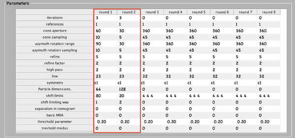
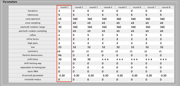
Everything is ready to create a new project. Below, the numerical parameters.
Fill in the input values, computational, and environment parameters for pr_0.
Launch it,
run aligment_for_reference.m
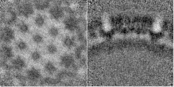
The last iteration average should look something qualitatively close to the one shown in the figure. To extract and plot the last average,
 aPath  =  ddb([ pr_0 ':a:ite=last']);
 a      = dread(aPath);
 dshow(a)
At this stage, with only one tomogram, the wild average (shifting mode 2 in the second round allows for this connotation) already reveals a strong c6 symmetry.
Extraction of first per tomogram average
Let us start by preparing the last average by running the prepare_average_for_chimera.m script.
re style="color: blue"> movefile([pathToDownloads '/Subtomogram_averaging/scripts/*'], './scripts') prepare_average_for_chimera(pr_0)
This function will simply filter via dynamo_bandpass, and invert the map.
To open the file into Chimera,
dynamo_chimera(theNameOfMyMap)
If for some reason is not able to find the application, just give Dynamo the path,
dynamo_chimera(theNameOfMyMap,'path',thePathToChimera)
The volumen viewer window will pop out.
Adjust the density threshold and, if helps, change the color.
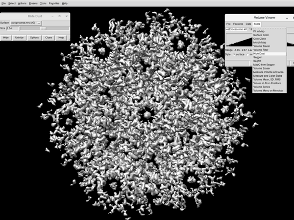
The second pre-processing step is to remove noise.
Go to Tools > Volume Data > Hide Dust.
Adjust the percentage until one unique blob is in the scene.
The density map is ready to be annotated:
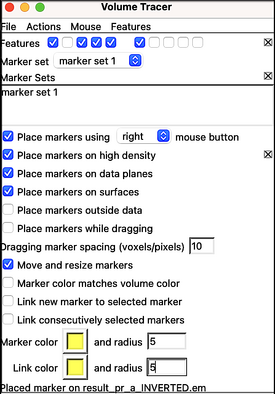
Open the annotation window inside Tools > Volume Data > Volume Tracer.
Create a new marker set via File > New marker set.
Select a proper configuration for marker placement.
Next, rotate the average upside down:
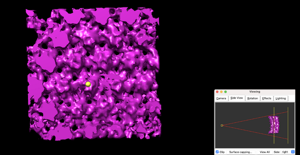
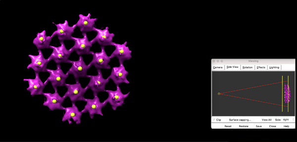
Select a proper perspective with the help of Tool > Viewing Control > Side View (check the figure below and pay attention to the slicing tool position).
Marking the tip of the CA-N terminal domain,
Define the center of unit cell with a marker.
Save them to disk:
Volume tracer: File > Save current marker set > 'reference_center.cmm'
From here, copy and open the first_aligment_per_tomogram.m script.
style="color: blue"> movefile([pathToDownloads '/Subtomogram_averaging/scripts_wc/*'], './scripts') open first_aligment_per_tomogram.m
As usual, change the paths and set up the available hardware resources,
Change paths.
Specify hardware resources.
Using the 'reference_center.cmm', the task you will need to complete is the centering and re-average of the particles.
Compute the vector pointing from box center to the new coordinate.
Create transformation object, and transform the table per se.
Re-average the particles (Do not forget Fourier compensation).
Of course, before launching an alignment project, you should perform a sanity check. To do this, visualise the volume before and after the centre and click on the corresponding coordinate.
dshow -otf aBeforeCentering
dshow -otf aAfterCentering

Pin the coordinate and compare.
From here, running the initial per tomogram alignment is straightforward. The configuration of the project is identical to the alignment for reference but from here on, imposing a c6 symmetry. Thus,
Configure the c6 symmetry on both rounds of the project.
Each project will take about 1 hour 30 min (estimation with 8 gpus). To directly run the script:
run first_aligment_per_tomogram.m
The results of the last iteration symmetrised average should look something qualitatively close to the ones shown in the figure. Visualise the results and compare against the one you have obtained.
aTsAll = [];
for idx = 1:nTomo
    aPath = ddb([pr_1{idx} ':as:ite=last']);
    aTsAll = [aTsAll; dread(aPath)];
end
dshow(aTsAll)
The first thing to notice is that each average is centred. Thanks to this operation, the periphery reveals more proteic units. The biologically most relevant feature is the hexameric intra-structure of Gag, which can be observed in each of the units for all tomograms. The differences found in each tomogram can be attributed to the inherent quality of the tomogram, the structural variety of the biological target (size, imperfections, degree of immaturity of the VLP), and the randomness of the inherent process that takes place during the alignment project.
Computing an average of averages
To complete this small project, open the corresponding aligment_for_average.m and change the paths inside,
open aligment_for_average.m
Change paths.
The configuration of the project is maintained from first per tomogram alignment. The difference lies in the data used. Here, as the names implies, all the tomograms averages will be merged onto one single average:
Create corresponding merged table, and set:
- No missing wedge compensation needed.
- Particle tag number = tomogram number
- Centers.
The motivation behind this computation is to minimise manual labour in the next step. It will run quickly (near 15 minutes 8 workers), since it only contains 5 particles. Launch the project by typing:
run aligment_for_average.m
To check the final average,
aPath = ddb([pr_a ':as:ite=last']);
dtmshow(aPath)
The symmetrised average should look something qualitatively close to the one shown in the figure.
Extraction of second per tomogram average
The average of averages is prepared as previously:
prepare_average_for_chimera(pr_a)
To open the prepared map inside Chimera,
dynamo_chimera(theNameOfMyMap)
This time, every 18-meric assembly of the capsid protein p24 are marked, so:
Volume tracer: File > New marker set
Mark the centers of every unit cell of the hexameric lattice
Save the  current marker set under 'particle_centers.cmm'.
The rest of this is implemented inside the script second_aligment_per_tomogram.m There are a lot of things going on for data preparation before running the alignment. Thus, it is worth diving into what is going on in detail.
We can use our previous results to set up an approach that centers the alignment on the individual. Each one of the particles in our new data set will be a subbox (a lattice unit cell) that we have just defined in the averages. The so-called 'subboxing technique will be used to redefine the area of interest inside a previously defined average.
In this example, the candidate coordinates will be determined using a two-step subboxing procedure. Note that, in principle, one subboxing step would suffice. However, this would have to be done for each tomogram individually. Therefore, the motivation behind the average of average computations is to minimise manual labour. Since the average is composed of multiple subvolumes with individual orientations, these coordinates can be then translated (or mapped) onto each of those subvolumes and finally also onto the tomograms themselves.
Let us now begin with the hands-on portion of the script:
open second_aligment_per_tomogram
The first step consists in mapping coordinates back onto the averages. Similarly to what was done for re-entering,
the vector from box center to new coordinate for each coordinate is computed. To complete this process,
Create a mini table for each average that contains the corresponding coordinates.
Merge the mini tables.
The second step involves mapping coordinates back onto the tomograms. Now, the vector from each average box center to the new subbox center is computed. Finally, as above,
Obtain the last subboxing table per tomogram.
Combine the tables into one.
The coordinates describing the same volume should be removed. Therefore,
Exclude the repeated unit cell.
Before cropping the particles, let us visualize the merged table generated containing the candidate positions before and after subboxing:
Add a break point in the line where ckpt variable is declared.
Run second_aligment_per_tomogram.m script section
About 5000-9000 coordinates per tomogram should have been defined. One table should suffice as a means of comparison:
docFilePath = [root '/catalogue/tomograms.doc'];
fileID  = fopen(docFilePath); D = textscan(fileID,'%d %s'); fclose(fileID); tomoID  = D{1,1}';
idx = 1;

tSubboxPath = ['subbox_' D{1,2}{idx,1}(end-7:end-4) '.tbl'];
tOriPath = ddb([pr_1{idx} ':rt']);

refs = {'Before', 'After'};
tbls = {tOriPath{1},tSubboxPath};

figure;
for i = 1:length(refs)
subplot(1,2,i);title([refs{1} ' subboxing: ' num2str(size(dread(tbls{i}),1)) ' particles.']); h = dpktbl.plots.sketch(tbls{i},'haxis',gca()); h.zlength.value=100;
end
We can complete the rest of the script. So, next, we will use those coordinates to extract a new set of subvolumes with a smaller sidelength.
Re-crop subboxed particles onto corresponding folder with a box size of 192.
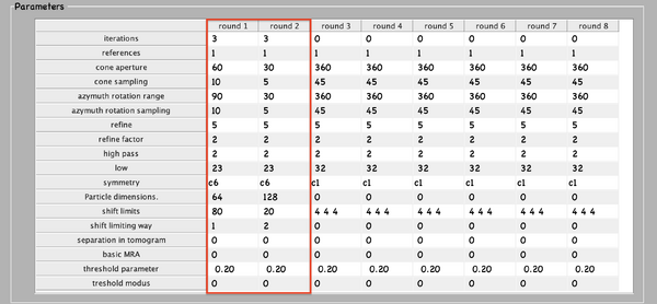
Prior to running the second per tomogram project, the subboxed particles are re-averaged, and save them to disk. Since we will need input templates for the incoming project. Its configuration is found below. If we compare this second configuration with the previous, the angular search space and shift limit is reduced. This is possible because particle positions are now more accurate. Recall that the hexagonal lattice structure inherent to the immature HIV-1 CA-SP1 is the target of the present localised alignment. Nevertheless, high resolution is not of interest yet. This is the reason why subvolumes are still binned on-the-flight.
This section, per tomogram, is estimated to take 30 minutes for the subboxing block (8 workers), and 3.5 hours for the alignment project (8 gpus). To actually compute the cropping of the particles and the corresponding alignment projects:
run second_aligment_per_tomogram.m
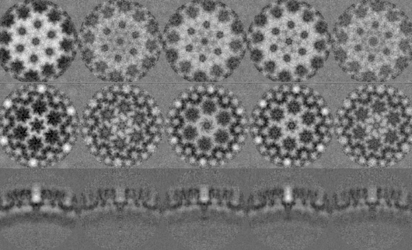
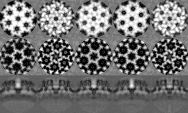
The results after running the project demonstrate how localised alignments are capable of driving the alignment robustly. To replicate the figure:
aTsAll = [];
for idx = 1:nTomo
    aPath = ddb([pr_2{idx} ':a']);
    aTsAll = [aTsAll; dread(aPath)];
end
dshow(aTsAll)
The higher contrast is associated with a stronger signal. This is important since a potential downside of this technique is the reduction of the amount of signal available to drive the alignment due to smaller box sizes. Therefore, is an indicative of a better estimation of their pose; a better concordance between particles (e.g. in the cavities between MA - CA , there is no density. In previous stages of the project, in these areas, there was uniformly distributed noise). Furthermore, in the orthoslice through the CA-SP1 region (last row), each unit of lattice locally morphology was previously fuzzy. Whereas now, the density is ordered and some helical patterns can be grasped.
Extraction of coarse half maps
This block is 100% automated. As we have been doing so far, some functionalities have to be implemented in order to be able to launch it.
Open the corresponding script:
open coarse_gold_standard_alignment.m
From the last project, the tables will be gathered. Column 10 stores the CC between each aligned subvolume and the final average. The exclusion process is done by fitting a Gaussian mixture model (GMM) to the such distribution. The MATLAB function fitgmdist will help to classify them into a combination of two populations. The one with the lower CC score is assumed to be the “bad” class (i.e., particularly bad quality or subvolumes containing pure noise). Therefore, it needs to be excluded from the processing. The threshold is then defined by taking the minimum between the 2 Gaussian peaks and by adding an empirically defined constant of 0.01.
While the table get filtered, to visualise the results add the following lines in the loop:
figure;
hold on;
histogram(t(:,10), 'Normalization', 'pdf', 'EdgeColor', 'none')
plot(x, pdf(gmdist, x'))
xline(thresh)
xlim([0 0.5])
legend('CC distribution','GMM fit','Threshold')
stackName{idx} = D{1,2}{idx,1}(end-7:end-4);
title(['Stack: ' stackName{idx}])
Tips:
You can activate the interactive mode by adding a `keyboard` command in your script, then type in your visualization on the terminal.
To terminate debug mode and continue execution, use the dbcont command.
To terminate debug mode and exit the file without completing execution, use the dbquit command.
Similarly to the subboxing section, is interesting to see how the filtering strategy worked. So:
Add a break point in the line where ckpt variable is declared.
Run coarse_gold_standard_alignment.m script section
For each stack of particles, the threshold determination and the fitted distributions in the graphs below.
Following filtering, a new average per tomogram is computed. In the next step, the height of every particle is homogenised to a common center unit cell. To ensure that, independently of the tomogram, the z-height should be consistent across sub-volumes. To this end a synthetic reference is derived from a model:
Compute a mask from a membrane object.
The object's properties, thickness, radius, and side-length are already changed. In practice, you will need to visualise what you are doing. So dview is what you are looking for:
dview theNameOfMyMask
Both, template and reference, are band-passed and all the particles are aligned against it. Remember, axis orientation and x/y-shifts are already consistent due to the imposed C6 symmetry. Thus, the only permitted shift is along z-direction:
Fill in the dalign allowing only 20 pixels of z-shift (flag: "lim").
Then, the resulting transformation parameters are applied to the table via dynamo_table_rigid. Again, fixing coordinates that describe the same particle and saving the table to disk.
Finally, all subvolumes containing one centered unit cell are re-extracted one last time. The side length is of 192 pixels is preserved. This time, per tomogram, about 2,000 to 5,000 particles are expected.
The point has been reached: the quality of the particles and their initial orientation are good enough to serve as the basis for a gold standard alignment. Prior to launching the project, as explained before:
Merge everything to a single container
Get even and odd index
Prepare each half template.
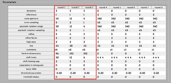
The configuration of the 2 independent alignment projects using the starting references that have been created before is displayed below. A total of 3 rounds with 3 iterations each are set up. The parameter search space is reduced after each round. The low-pass filter is increased to 32 pixels (8.1 Å), and the last 2 rounds are run on full-sized particles.
The estimated times are, for registration, and re-cropping, 20 min (8 workers). The coarse even/odd project is around 48 hour per half-set (8 gpus). Therefore, if you have already completed the task filling in the missing parts:
run coarse_gold_standard_alignment.m
To check the resulting maps:
aEPath = ddb([pr_EO{1} ':as']);
aOPath = ddb([pr_EO{2} ':as']);
dshow([dread(aEPath); dread(aOPath)])
Extraction of refined half maps
The script refined_gold_standard_alignment.m is responsible for refining previous results by pruning again the dataset and running a final alignment project with adapted parameters.
Open the corresponding script:
open refined_gold_standard_alignment.m
This time, to remove particles of low quality, the dataset is reduced through a normalised, per tomogram, CC filtering. The reason for thresholding separately is to avoid reducing the coverage of the zeros of the CTF. The risk emerges from different defocus values of the tomograms influencing the overall CC score. With the help of dpksta.filters.byCC, subvolumes with a score lower than 1 standard deviation below the mean are removed. This function performs normalisation by the angle of latitude. This is important, since particles at the poles of the VLPs generally have a lower CC score than particles on the equator due to missing wedge effects. More precisely, this function works by fitting the first 2 terms of a general Fourier series to the data. As usual, after the tables are pruned, a new average is computed that will serve as reference for the last alignment project.
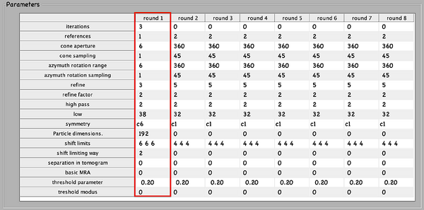
For this 2 projects configuration the set up is the same parameters as the last round of the previous project but with a stricter low-pass filter up to 38 fourier pixels (~ 6.8 Å). Although, the intuition is that there is still room for improvement in terms of resolution. Therefore, the last bullet is to focus the refinement more onto the area of interest.
For this, the idea is to create a tighter mask. While one option is to draw the mask by hand, the choice is to exploit the already existing motives in dynamo (as last time, there is trial and error until the properties satisfy you biological target). For target the capsid:
Create a custom tight mask as the intersection of a membrane (parameters given), and a cylinder ( radius : 87; size : 192; position : [97 97 97]).
Be aware that the default mask option is still used. The new mask is overwritten via dvput(theNameOfMyProject,'file_mask',theNameOfMyMask).
The computation time of this for the refinement project is estimated to be 24 hours per half-set (8 gpus). Launch it via:
run refined_gold_standard_alignment.m
Et voilà! The latest results have been obtained. And with them, we have finished the subtomogram averaging projects.
Finally, the resulting odd/even maps are reformatted and prepared. To this end, the even half-map is aligned to the odd half-map with the usual function dalign. The resulting transformation parameters are used to transform the table corresponding to the even half-map though dynamo_table_rigid. The table is then used to re-average the even particles usingdaverage imposing a c6 symmetry, dynamo_csym.
The reason for this re-averaging is to avoid edge artifacts caused by the half-map alignment. Then, they are saved (dwrite) according to RELION convention so that they can be used for the gold standard Fourier shell correlation (FSC) computation. This is important, since unless the map's name starts with ‘half1_*.mrc’ and ‘half2_*.mrc’. Else, RELION will not be able to parse them.
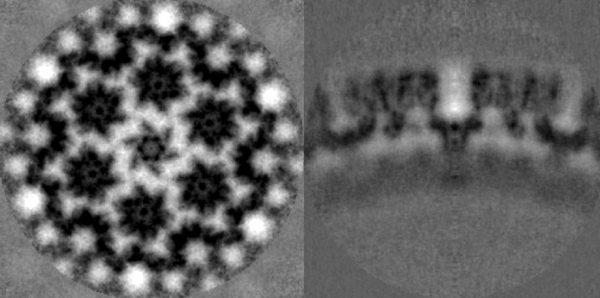
A final density map is additionally computed by re-averaging all particles of the full dataset. This isosurface visualisation is displayed below. Note the necessity of re-averaging to ensure a correct Fourier compensation of the final map. Therefore, the corresponding flag, fc is set to true (daverage(nameOfTheStarFile,'t',dynamo_table_merge({theNameOfHalfMapEven, theNameOfHalfMapOdd}),'fc’,1)). Then, simply:
dynamo_chimera(theNameOfMyFinalMap)
Outputs
- Final high-resolution dynamo average.
- Two high-resolution half-maps.
- Particle table of high-resolution dynamo average.
Fourier shell correlation
Initial comments
At the end of a gold-standard alignment, we can estimate the resolution of the final average by comparing the Fourier shell correlation (FSC) of the two half-maps.
An FSC mask should be generated to limit the FSC computation to the areas where the protein densities are present. A better FSC mask can be used to deduce better resolutions, but a poor FSC mask can either deduce a worse resolution or even an artefactual resolution.
So this analysis can be divided in two steps: the FSC mask creation and the actual FSC computation. Both of these steps can be done either in dynamo or in RELION. In this walktrough the alignment mask will be generated in dynamo and the FSC computation will be done in RELION.
This choice was made because the mask creation in RELION (using the Mask creation job) can limit the user freedom. In fact, it will always be a Gaussian filtering and binarization of an input density map.
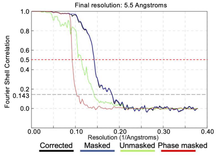
On the other hand, the FSC computation in dynamo using the dynamo_fsc function will only compute the FSC curve (https://www.dynamo-em.org/w/index.php?title=Fourier_Shell_Correlation). RELION Post-processing job will calculate the phase randomized FSC in addition to the usual FSC.
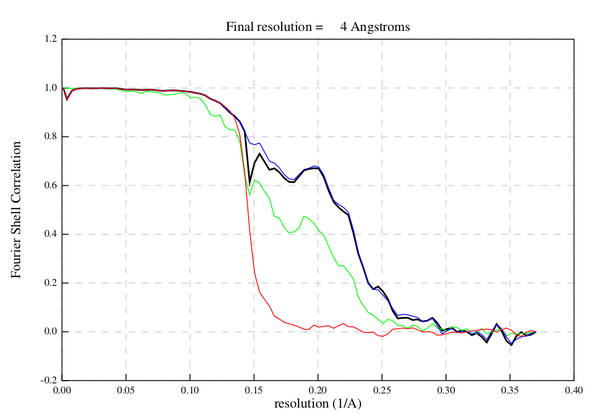
Here is an example of an FSC computation using RELION on a different dataset. Note the effect of the mask on the FSC curve.
In general, an healthy FSC computation will have the following characteristics:
- RELION assigns the final FSC close to the FSC of the masked half-maps (blue line, see legend).
- The phase randomized FSC (red line) will go to zero quickly.
- At high frequency all FSC curves will go to zero.
We must take care to note the behavior of all of the FSC curves. Some typical causes of unhealty FSC curves can be: unmasked symmetrization artefacts, sharp edges caused by the FSC mask or duplicate particles in the average.
Input
- two half-maps generated using the gold standard protocol.
Practical notes
The FSC computation will be done using RELION. Additionally, the script FSC_mask_generator.m will be used to generate the FSC mask.
Change the root
The even and odd averages found through dynamo have been precomputed. You can load them:
h1 = dread([root,'data/Dynamo_final_results/half1_final_reaveraged_unfil_ctf_corrected_thick_tomos.mrc']);

h2 = dread([root,'data/Dynamo_final_results/half2_final_reaveraged_unfil_ctf_corrected_thick_tomos.mrc']);
You can inspect the differences between the two half-maps by:
dshow(abs(h1-h2));
You should see something like:
Now we can start to build the mask.
Inspect a half map and determine the dimensions and center of cylinder that would contain the middle "wineglass" structure.
Generate a cylindrical mask:
mask = dcylinder([35,35],192,[96,96,126]);
And compare it with the half-maps:
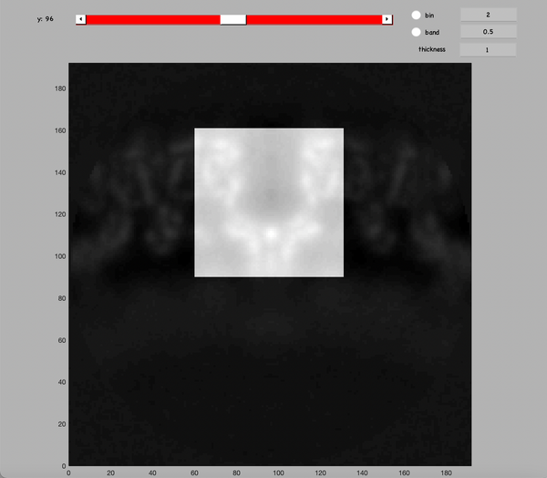
dshow(h1+mask)
You should see something like:
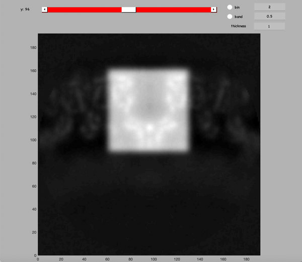
As mentioned in the initial comments, the mask will be mollified to avoid sharp edges. Remove them and inspect the result:
mask_m = dynamo_mollify(mask,3);
dshow(h1+mask_m)
You should see something like:
The FSC mask will be created using the usual dwrite command followed by the dpkio.tomo.mrc.setPixelSize command to set the appropriate pixel size in Angstrom in the header of the mask .mrc file. Copy the half-maps too:
px_size = 1.35;

dwrite(mask_m,'FSC_mask.mrc');
dpkio.tomo.mrc.setPixelSize(px_size,'FSC_mask.mrc');

dwrite(h1,'half1.mrc');
dwrite(h2,'half2.mrc');

dpkio.tomo.mrc.setPixelSize(px_size,'half1.mrc');
dpkio.tomo.mrc.setPixelSize(px_size,'half2.mrc');
Now RELION will be used to estimate the resolution. The RELION job to do this analysis is the Post-processing job.
Some relevant RELION documentation can be found in:
https://relion.readthedocs.io/en/release-4.0/STA_tutorial/Postprocess.html
https://relion.readthedocs.io/en/release-4.0/SPA_tutorial/Mask.html
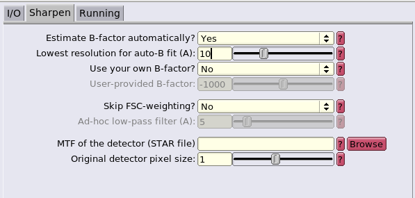
In this case, we will use the the generated FSC mask and ask RELION to estimate the sharpening B-factor automatically.
Note that the two half-maps need to be in the same folder and follow the naming convention: 'half1_XXXX.mrc' and 'half2_XXXX.mrc'. It may be necessary to rename the two half-maps to be able to set them in RELION.
load RELION4 with relion --tomo
Click to the Post-processing window
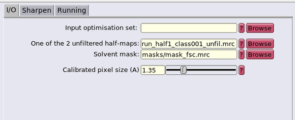
You will see the following GUI:
Fill in the GUI with half1.mrc as the map and FSC_mask.mrc as the FSC mask.

Set the pixel size at 1.35 A and the press Run!

Inspect the result by using the RELION GUI Display option of the logfile.pdf
The sharpened final average is saved as the postprocess.mrc file in the Postprocess job folder that RELION just created.
Outputs
- FSC curve.
- The corresponding FSC mask.
RELION conversion
Initial comments
RELION has some very interesting capabilities that can be used to complement dynamo. In particular, RELION 3d auto-refine job type is useful because it allows to run the equivalent of dynamo STA on locally back-projected particles. One advantage of this approach compared to cropping particles from the tomograms is that RELION can exploit explicitly the information that each particle is, in fact, a reconstruction based on information of multiple patches. However, a more immediately practical advantage is that RELION does not need to store in memory all of the full-scale tomograms.
Some disavantages of RELION are that it needs relatively good initial particle positions to start a 3d auto-refine job correctly and that RELION allows for less control on the angular alignment search spaces that dynamo. In addition to this, RELION is not meant to receive reconstructed tomograms as inputs, but instead it requires the unaligned tilt series to allow for the local back-projection procedure. This means that RELION also needs to receive the alignment parameter of the tilt series as well as CTF and dose information, which can be confusing to implement in practice.
However, these disadvantages can be removed by using the dynamo-RELION conversion tools. Two main tools are used in conjunction:
- a tomogram.star generator: this script will use the results of the dynamo fiducial-based tilt series alignment to create a file for RELION that allows it to link together the tilt series alignment parameters, the CTF parameters, the dose information, the microscope information and the paths to the unaligned tilt series.
- a particle.star generator: this script converts a dynamo particle table in a RELION-readable format. This allows RELION to start its 3d auto-refine with particles that of sufficient quality.
By using these tools users of dynamo can exploit the functions available in RELION. In this case, RELION will be used to refine the average generated by dynamo.
Other interesting ways to exploits the dynamo<->RELION converters can be:
- reconstructing only binned tomograms with dynamo and generate an initial set of particles. Next, refining the unbinned particles in RELION. This approach allows for not needing to reconstruct all of the full-sized tomograms. Indeed, for large datasets and depending on the resources available, it might not be practically possible to store in memory all of the full-sized tomograms.
- By converting the particles from RELION to dynamo, a user can exploit the dynamo functionalities that are not available in RELION, both in data analysis and visualization.
Input
- the unaligned, not dose weighted, not CTF corrected tilt series.
- the AWF folder paths.
- the CTF information.
- the dose information.
- the microscope parameters.
- a particle table.
Practical notes
The dynamo-RELION will be done using the script convert_data.m. Firstly, the script will recover the CTF information, the dose information, the microscope parameters and the alignment parameters previously computed and will generate a tomogram.star file. This file allows RELION to know how to locally reconstruct subtomograms directly from the unaligned, not dose weighted, not CTF corrected tilt series.
Change the root of convert_data.m
You can see that the first part of the script are the path to all the files required. RELION implicitly handles dose weighting, ctf correction, tilt series alignment and local reconstructions, so RELION needs access to this information. RELION has an implementation to automatically do this but only for IMOD output folders. A custom function to do the same with dynamo alignments is used in the script convert_data.m.
The RELION also need the microscope parameters.
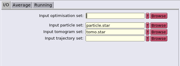
Update the parameters of convert_data.m
The second part of the script convert_data.m will convert dynamo particle table in a particle.star file that is meant to be compatible with the previously generated tomogram.star file. A particle.star file is paired with a tomogram.star file in similarly to how a dynamo particles table is paired with a dynamo catalogue of tomograms.
Try the conversion:
run convert_data.m
Two files have been generated: particles_converted.star and tomogram_converted.star.
Inspect tomogram_converted.star:
open('tomogram_converted.star');
The script is divided in 6 parts: an header and 5 tomogram blocks. The header includes the information of the microscope parameters as well as the location of the raw tilt series. Each tomogram block is split in as many lines as micrographs present in that tilt series. Each lines encodes the alignment parameter, the ctf parameters and the dose.
Inspect particles_converted.star:
open('particles_converted.star');
You will see the files has an header as well as a body with as many lines as particles. Each line includes the alignment parameters of a particle and the identification of which tilt series generates that particle.
From here on everything can be done with RELION. For example, the particles can be shifted in Z so that the GAG layer will be centered. Do this with:
system('relion_star_handler --i particles_converted.star --o particles_converted_shifted.star --center --center_Z 32');
Outputs
- a tomogram.star.
- a particle.star.
Final RELION refinement
Initial comments
As said in the previous section, RELION will be used to refine the average generated by dynamo. Since now the converted star file have been generated, all of the folowing steps are done in RELION.
RELION will be used to locally backproject the particles, create an initial template and run a 3d auto-refine project. These are the RELION equivalent steps of the dynamo steps of particles cropping, particle averaging and STA.
This step is strongly inspired by the RELION Subtomogram tutorial: https://relion.readthedocs.io/en/release-4.0/STA_tutorial/index.html. In particular the "Make pseudo-subtomograms", "Reconstruct particle", "High-resolution 3D refinement" and "Masks & Postprocessing" steps. Inspection of the RELION Subtomogram tutorial can be used to find how other RELION tools can be used to improve the reolsution even further. However, in this workflow, only the basic RELION steps will be expoited.
Input
- the tomogram.star.
- the particle.star.
- The usual FSC mask.
Practical notes
The Reconstruct particle job will be the first step. This will generate the template for the alignment.
The inputs will be the tomogram.star and the particle.star generated previously and the template will be generated of size 192x192x192 unbinned pixels by local back-projection of 2D patches of dimension 512x512.
The following steps indicate how to set up the RELION job.
open the relion4 tomogram GUI (relion --tomo)
Click on the relion4 tomogram GUI Tomo reconstruct particles
It will appear like this:
Fill in the tomogram.star and the SHIFTED particle.star that was created in the previous step.

A version of these star files was precomputed and can be found in:
data/RELION_initial_starfiles/tomo.star
data/RELION_initial_starfiles/particle_zp32.star

Then go on the Average page
It will appear like this:
Set the parameters like in the previous figure

Go on the Running page

This is where you can set the computing resources available to RELION.

Once this is done, click the Run! button.
The generated merged.mrc average should present the general structure of the GAG. It should look like the left-most average of the following figure:
The creation of all of the particles is done with the Make psuedo-subtomos job. The same size as the template are used.
This Make psuedo-subtomos step is described here put will not be done because of time limitations
A RELION job can be chained by giving as input of a job the optimisation set of a previous completed job.
Finally a 3D auto-refinement job can be started. The following parameters can be given:
This Refine3D step is described here put will not be done because of time limitations. This step took 18h on 8 GPUs and the computed reusults are provided in the folder:

data/RELION_final_results/refinement
data/RELION_final_results/postprocess
- the reference can be band-passed at 12 A. A non-bandpassed reference could generate artefacts.
- the reference will be C6.
- a convenient Mask diameter is 230 A. This created a spherical mask that is used in addition to the alignment mask.
- an initial angular sampling of 3.7 degrees and an initial offset range of 5 pixels with step of 1 pixel.
- If possible, GPU computing should be used with the identifications of all GPUs
The final refined and postprossed average can be found:
relion_refined_average = dread([root,'data/RELION_final_results/postprocess/postprocess.mrc']);
Open the [root,'data/RELION_final_results/postprocess/postprocess.mrc'] file with Chimera, set the step to 1 and use the tool/Hide Dust function to clear the view.
Outputs
- two half-maps generated using the gold standard protocol in RELION.
- the FSC curve.
- the high-resolution average RELION.
- the aligned particle positions in RELION.
