Walkthrough on manual marker clicking (EMBO2023)

This walkthrough describes the tools to manually locate fiducial markers for tilt series alignment using different graphical tools. Automatic alignment is described in Walkthrough on GUI based tilt series alignment and Walkthrough on command line based tilt series alignment .

Note : the reader should be aware that the working tilt series does not correspond to the ones used in the figures.

Data set

This tutorial uses one item from the EMPIAR dataset entry 10164 (https://www.ebi.ac.uk/empiar/EMPIAR-10164/).

Such tilt series has already been prepared (i.e., binned) and can be found by following the next steps.

Open a new local terminal and navigate to the directory where the tutorial dataset and project should be located.

 d/embo2021/u/emboXX/prac-5

Inside this folder, the file needed is bs001ts001.mrc.

The dmarkers GUI

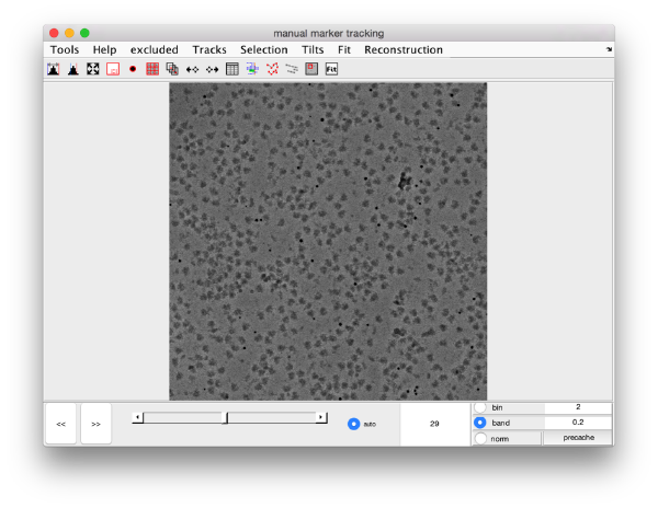
This GUI is the basic tool for exploring tilt series and annotating on it using Dynamo. It allows to edit manually positions of markers, to fit them to a projection model, and to create an aligned data stack and a reconstruction based on this fitting.

Loading the data

First, it is convenient to inspect the tilt series:

ts = dread('b001ts001.mrc');

Then, pass the variable to the gui dmarkers:

 gui = dmarkers(ts,'tiltAngles',-57:3:60);

here, gui is just a handle to the GUI. This handle can be used on a later point to operate on it. Note that we also need to pass the tilt angles, as they will be needed for fitting a projection model.

dmarkers GUI

Basic visualization controls

Slide on micrographs

• Use the slide bar to view a transition of the micrographs (lower resolution images will be shown during the transition, full resolution images will be shown )
• left and right arrows move the previous or next micrograph in the tilt series.

Zoom

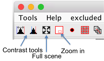
• You can zoom into a point by using the wheel.
• The small red window in the tool bar can be used as magnifying-glass to zoom in into a hand-draw a region.
• The tool with the four arrows pointing into the corners zooms out of the scene totally.

Basic controls inn dmarkers GUI

Dragging

The scene gets dragged by moving the mouse while keeping pressed the right mouse button.

Elimination of defective tilts

Some micrographs may be defective because of errors during acquisition. They can be markers as invalid by the key x. If you want to undo the marking of a micrograph as invalid, use shift+x.

Initiating a trace

A three-dimensional gold bead is represented by a trace. A trace is a set of observations, where we call observation to the location of the projection of a gold bead in a given micrograph.

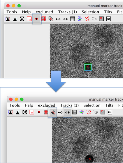
The tool with a black point and a red edge starts the trace initiator. The cursor in the GUI becomes a cross; while this cursor is active, clicking on the screen will create a new gold bead.

Following a trace

To select a gold bead, click on it with the mouse, a green box will appear on the observation corresponding to the selected markers in the current micrograph. Important: to add observations into a trace that you have just created, you need to select it, otherwise your next clicks on the screen will be assigned to the trace that is currently under selection.

Once you have selected a gold bead, you should switch off the tool for adding gold beads, and switch on the tool for adding observations to the gold bead currently under selection. The icon represents a point being tracked across several micrographs.

You can use the arrows to move to the next or previous micrograph after clicking the gold bead.

Additionally, you can connect the click and right or click and left tools. When they are switched on, after a click on the screen, the GUI will automatically move to the next micrograph.

The gold bead click tools sets new traces, the track tool allows adding new observations to the currently selected trace

Key controls during clicking

• d will delete the closest observation (point in currently shown micrograph).
• shift + d will delete a full trace.
• m will move the observation of the currently selected shape to the location of the cursor.

Auxiliar views during clicking

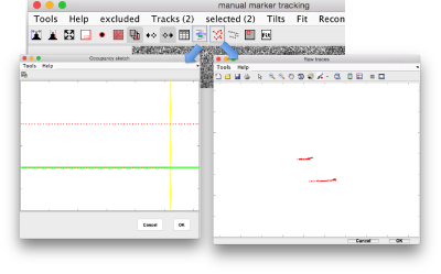
There are two auxiliary GUIs that can be used to control the growth of the traces based as you click the points. The occupancy window updates as a new observation is added into a gold bead, showing the current content of each trace. And additional control shows the content of each trace as new points are clicked inside.

Tools to follow the traces across the micrographs

Saving the marker set

We want to save current set of markers into disk, by using the save to disk option in the Tracks menu. This will create the file Tracks.dms in disk.

Fitting to an alignment model

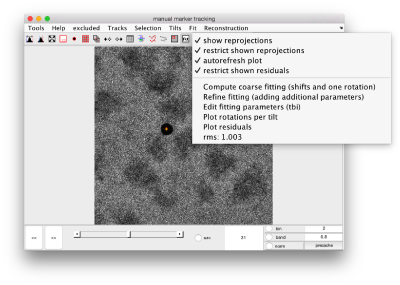
When you have enough observations, you can proceed to fitting the location of your gold beads to a projection model. The tool with the icon Fit will compute a set of shifts and a single angle psi of rotation for the tilt axis.

In the Fit menu on the GUI, you can find the current error, i.e., the mean residual between each observation and the projection estimated by the fitting model.

Fitting menu in dmarkers

Extended fitting models

In a coarse fitting, Dynamo only tries to solve for shifts and a single rotation angle for all micrographs. It is possible to refine this fitting allowing a different rotation of the tilt axis for each micrograph. You can select for a richer model that computes for one different rotation angle on each micrograph by checking the option eachTilt on the parameter psi (default is single).

Although you will get a lower error value, this might be due to overfitting. Thus, richer parametric models should not be used if you don't have enough markers on each micrograph (in the order of the tens.)

Reconstruction through the command line

Creating reconstructions through the command line is convenient when organizing the processing of batches of tilt series. Automatic selection of markers is explored in a different walkthrough, here we describe the command line tools for creating reconstructions once a marker set is available. The steps are:

• Fitting of the available markers (using a fitter object).
• Extraction of alignment parameters (using an aligner object).
• Creation of an aligned tilt series.
• Weighting the tilt series appropriately for a weighted-back-projection or Sirt-like reconstruction.
• Creation of the tomogram through back projecting the filtered aligned stack.

If you have a set of markers saved in a file in disk, you can load it to memory through:

markers = dread('Tracks.dms');

Then, you can create a fitter object:

fitter = dfitter(markers);

This object needs to know where to put the rotation center of the aligned tilt series.

fitter.setCenter(ts);

and prepare it to run with standard parameters:

fitter.physical.defaultInitialization();

The command

fitter.linearScan();

will then compute the best psi angle for the rotation of the tilt axis together with the shifts. They can be gathered into an stack alignment object

stackAligner = fitter.getStackAligner();

that gets then applied onto the original tilt series in the variable ts.

tsAligned  = stackAligner.applyOnStack(ts); 

This aligned stack can be visualized through:

dtmshow(tsAligned);

Binned reconstruction

A reconstruction with a bigger pixel size can be computed by resizing both tilt series and markers. A marker object can be resized through:

markersBinned = markers.math.bin(2);

Here, the factor 2 indicates that the coordinates of the markers get halved twice. This factor needs to be applied also to the tilt series:

tsBinned = dpktilt.bin(ts,2);

Now, we can refit the binned markers, proceeding as above:

binnedFitter = dfitter(markersBinned);
binnedFitter.setCenter(tsBinned);
binnedFitter.physical.defaultInitialization();
binnedFitter.linearScan();
binnedAligner = binnedFitter.getStackAligner();
tsBinnedAligned = binnedAligner.applyOnStack(tsBinned);

To create a weighted back projection reconstruction, this stack needs to be weighted with a ramp function in the Fourier space.

 tsBinnedRamp = dpktomo.rec.applyRampFilter(tsBinnedAligned);

Then, we can use the command dpktilt.math.backproject to create a reconstruction.

 fbp = dpktilt.math.backproject([400,400,400],tsBinnedRamp,-57:3:60,'mw','*'); 

Here, the flag 'mw' is merely instructing Dynamo to use all available cores.

In case you did not mark a bead on every tilt you might get an error message at this point. Ideally you would go back and either mark at least one bead on the corresponding tilt or, if there are no good beads, you would exclude the tilt. Alternatively (but not recommended) you can use the following command to exclude the tilts without marked beads from the reconstruction:

 fbp = dpktilt.math.backproject([400,400,400],tsBinnedRamp,fitter.physical.thetas(fitter.physical.indicesActiveTilts),'mw','*'); 

The reconstruction object fbp contains the reconstructed tomogram in its property .rec, which can be visualized through:

dtmshow(fbp.rec);