Walkthrough on vesicle models
This walkthrough is a step-by-step guide that teaches how to extract subtomograms from vesicle-like structures using the Dynamo vesicle models.
Data
We are going to demonstrate the basic ideas and tools on a synthetic dataset. This data is already available in the catalogue manager. It can be accessed by first opening the catalogue manager using the command:
dcm
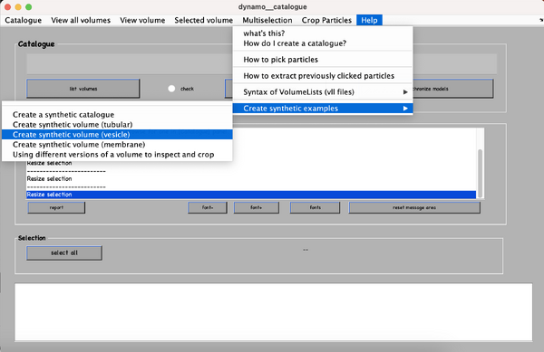
After the catalogue manager opens, we create the synthetic tomogram that includes a spherical surface (vesicle) in the following way:
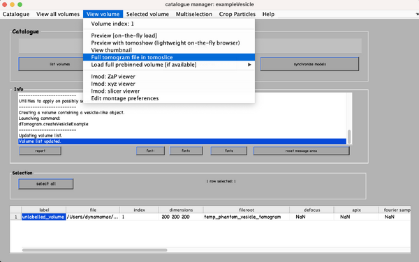
A new tomogram entry appears in the catalogue manager. Any further annotations (models) to the tomogram will be linked to this entry. Select the entry and open it:
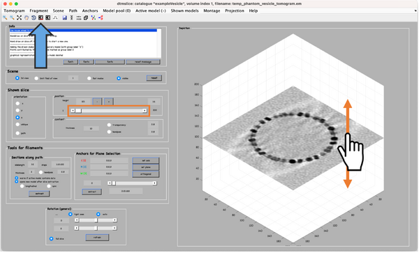
A tomogram viewer opens. You might need to adjust the contrast (blue arrow). To move through the tomogram slices, you can either use the mouse wheel, click and drag the tomogram slice up and down (orange arrows), or move the position control left and right (orange box).
Manual annotation
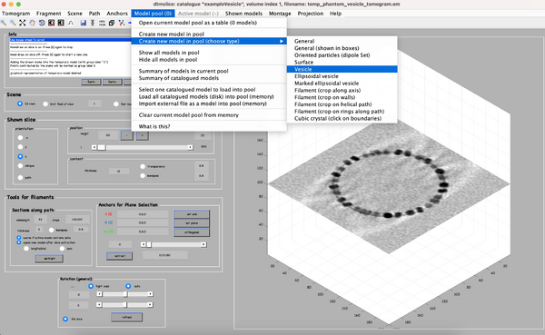
The annotation of the vesicle-like surface is done within a so called model. We open a new model of type vesicle as follows:
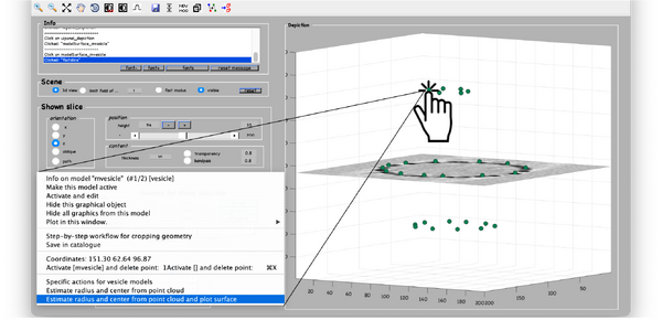
Once the model is created an active, we can navigate in the tomogram. Now, manually add model points along the surface of the vesicle. To do that, first move the slice up to a high z height. Then place the mouse cursor on the membrane and press the key [c] on your keyboard. This adds a new model point. Continue adding model points as shown below. Use the right-click to delete points if needed. Three layers are normally enough. Note: A known bug may cause the clicked points to be generated slightly displaced from the mouse cursor. Maximise the window of the tomogram viewer to get rid of this effect.
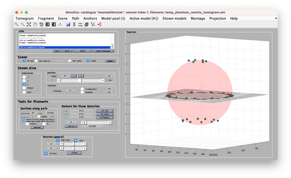
Now, we just need to invoke the method that fits the center and radius properties of a vesicle given a cloud of points. From the command line, this method is called approximateGeometryFromPoints. In the browser dtmslice we can invoke it directly by secondary clicking on one of the points of the model and selecting the option for fitting and plotting.
A transparent surface should be visible, allowing you to judge the quality of the fitting quickly sliding the slice up and down.
Generate subtomogram coordinates
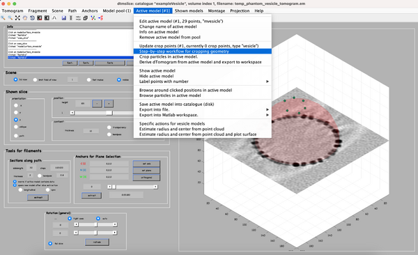
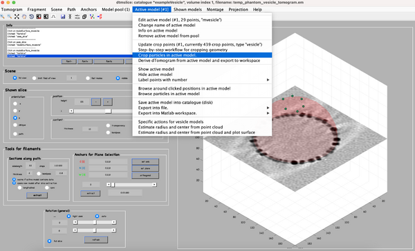
Using the clicked model we can now define the coordinates where the subvolumes will be extracted. To do that, we first processes the clicked model points using the model workflow to generate a user specific cropping geometry. Open the workflow:
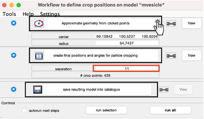
You get a new window with the model workflow. It has 3 large buttons, squared on black, that are executed sequentially starting from top. First, the same method used previously fits the center and radius properties of the vesicle given a cloud of points. However, after the big button is pressed, the model parameters are updated.
In this case, our synthetic sample has little to offer biologically. Upon initial examination, no symmetry in its patterns is observed. Hence, the most interesting strategy seems to be to select each unit as a single cropping point. This is the reason of selecting a separation of 11 pixels (parameter squared in red). The number next to # crop points (in this example 439) shows the total number of subvolumes that will be cropped. After you typing the new sampling distance, press the second big button.
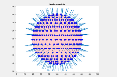
This will create equally distributed control points and estimate an orientation for each position. To visualise, click the viewing options bellow.
As you can see, each point has its own orientation. The shown orientations represent the z-axis of the particles that will be imposed by the model. Where the z-axis is set to be normal to the vesicle surface:
Save the model by clicking on the third big button, save resulting model into catalogue, and we can move to the subtomogram extraction.
Extract subtomograms
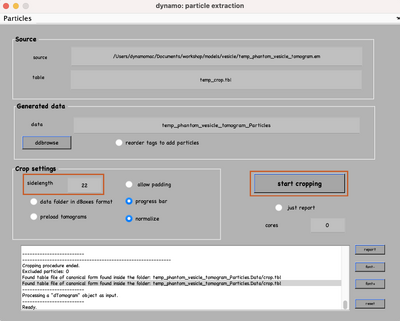
In this final step we extract subvolumes at the coordinates defined before. First, open the particle extraction GUI:
Set the sidelength to 22 and click on start cropping (orange boxes):
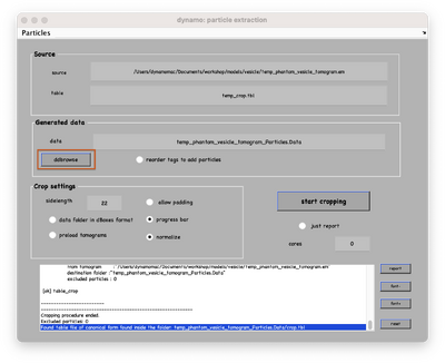
To see the results, click on ddbrowse (orange box):
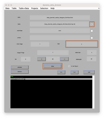
In the new window activate the table, select the x-axis and click on show (orange boxes):
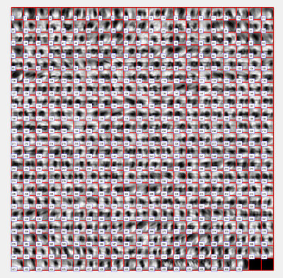
These are 2D representations (projections) of the actually cropped 3D subtomograms.The lack of a repeating pattern, coupled with the distribution pleiformism, does not allow each of the cut-off points to always coincide at an individual target's centre of mass. Yet, the box size is sufficient to collect, albeit off-centre, at least one of these inside the box. Therefore, these particles are susceptible to be aligned.
Indeed, to identify individual targets, it may be more convenient to use a general Dynamo model, create template(s) and make the classical query to tomogram space.
