Difference between revisions of "Walkthrough on GUI based tilt series alignment"
| Line 95: | Line 95: | ||
[[ File:alignGUI_markerSetsCanBeViewedAsCloudOfPoints.png |thumb|center| 600px|marker sets can be viewed as cloud of points]] | [[ File:alignGUI_markerSetsCanBeViewedAsCloudOfPoints.png |thumb|center| 600px|marker sets can be viewed as cloud of points]] | ||
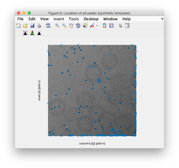
| − | This view shows the x,y coordinates of ''all'' cross correlation peaks on | + | This view shows the x,y coordinates of ''all'' cross correlation peaks on all the micrographs in the tilt series. |
[[ File:alignGUI_cloudOfUnindexedCcPeaks.png |thumb|center| 600px|cloud of unindexed cc peaks]] | [[ File:alignGUI_cloudOfUnindexedCcPeaks.png |thumb|center| 600px|cloud of unindexed cc peaks]] | ||
| + | We can also check the positions of all the detected spots on each micrograph: | ||
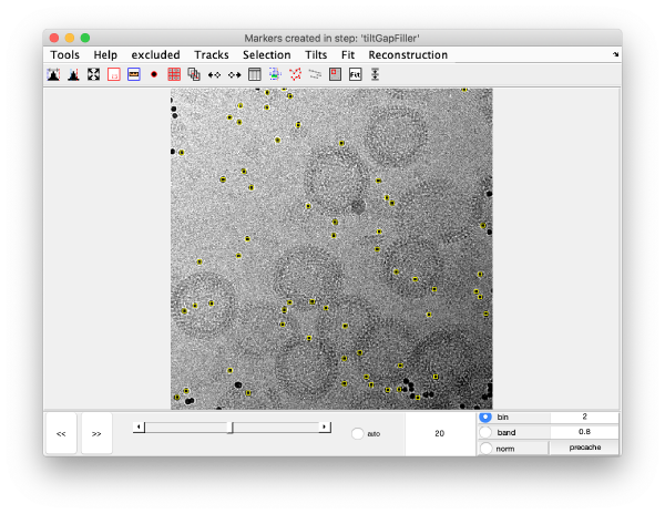
[[ File:alignGUI_showsTheDetectedSpotsOnTheVideoGUI.png |thumb|center| 600px|shows the detected spots on the video GUI]] | [[ File:alignGUI_showsTheDetectedSpotsOnTheVideoGUI.png |thumb|center| 600px|shows the detected spots on the video GUI]] | ||
| + | This GUI does not allow for edition of the markers. | ||
[[ File:alignGUI_staticVideoAnnotationsCannotBeEdited.png |thumb|center| 600px|static video annotations cannot be edited]] | [[ File:alignGUI_staticVideoAnnotationsCannotBeEdited.png |thumb|center| 600px|static video annotations cannot be edited]] | ||
| + | The neighbourhood of cross correlation peaks can be visualised individually: | ||
[[ File:alignGUI_EachPatchWillBeAPutativeGoldBead.png |thumb|center| 600px|Each patch will be a putative gold bead]] | [[ File:alignGUI_EachPatchWillBeAPutativeGoldBead.png |thumb|center| 600px|Each patch will be a putative gold bead]] | ||
[[ File:alignGUI_theSetOfCcPeaksIsShownAsAMontage.png |thumb|center| 600px|the set of cc peaks is shown as a montage]] | [[ File:alignGUI_theSetOfCcPeaksIsShownAsAMontage.png |thumb|center| 600px|the set of cc peaks is shown as a montage]] | ||
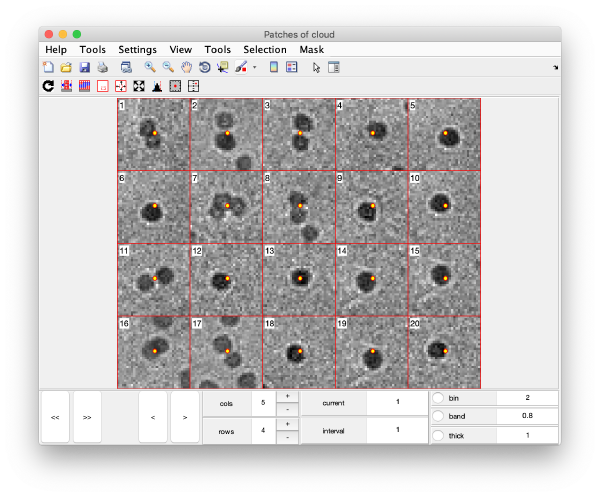
| − | [[ File:alignGUI_exampleOfFailedSearch.png |thumb|center| 600px|example of failed | + | This visualization is normally a good gauge on how the detection procedure has worked. The example below would be an example of detection procedure carried with wrong search parameters |
| + | [[ File:alignGUI_exampleOfFailedSearch.png |thumb|center| 600px|example of failed gold bead detection]] | ||
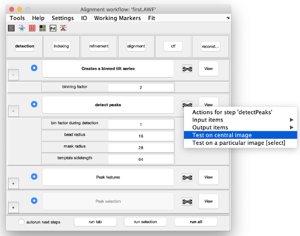
| + | Note that you have the option of testing your parameters against a single image before launching a full detection procedure. | ||
[[ File:alignGUI_toolboxOptionForTestingTheParametersOnACentralImage.png |thumb|center| 600px|toolbox option for testing the parameters on a central image]] | [[ File:alignGUI_toolboxOptionForTestingTheParametersOnACentralImage.png |thumb|center| 600px|toolbox option for testing the parameters on a central image]] | ||
[[ File:alignGUI_resultsOfTestingOnACentralImage.png |thumb|center| 600px|results of testing on a central image]] | [[ File:alignGUI_resultsOfTestingOnACentralImage.png |thumb|center| 600px|results of testing on a central image]] | ||
=== Computation of observation features s=== | === Computation of observation features s=== | ||
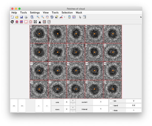
| + | At this stage, the observed cross correlation peaks are analysed. In the current ''Dynamo''' version a merit figure is assigned to each peak based on a "rotational merit" that measures its similarity to a circle. The results can be depicted on patches representing individual gold beads: | ||
[[ File:alignGUI_patchGalleryForFeatures.png |thumb|center| 600px|patch gallery for features]] | [[ File:alignGUI_patchGalleryForFeatures.png |thumb|center| 600px|patch gallery for features]] | ||
[[ File:alignGUI_theGalleryAllowsRelatingAppearanceOfGoldBeadAnValueOfTheFeatures.png |thumb|center| 600px|the gallery allows relating appearance of gold bead an value of the features]] | [[ File:alignGUI_theGalleryAllowsRelatingAppearanceOfGoldBeadAnValueOfTheFeatures.png |thumb|center| 600px|the gallery allows relating appearance of gold bead an value of the features]] | ||
| + | or extracting properties of the whole data set. | ||
[[ File:alignGUI_featurePlotterAllowsCheckingOfTheFeatureValuesOnTheWholeSet.png |thumb|center| 600px|feature plotter allows checking of the feature values on the whole set ]] | [[ File:alignGUI_featurePlotterAllowsCheckingOfTheFeatureValuesOnTheWholeSet.png |thumb|center| 600px|feature plotter allows checking of the feature values on the whole set ]] | ||
[[ File:alignGUI_differentPlottingOptions.png |thumb|center| 600px|different plotting options ]] | [[ File:alignGUI_differentPlottingOptions.png |thumb|center| 600px|different plotting options ]] | ||
| Line 115: | Line 122: | ||
=== Selection of best gold beads=== | === Selection of best gold beads=== | ||
| + | The cluster with the best markers is then selected. The individual patches can be inspected | ||
[[ File:alignGUI_checkObservationCloudAfterSelectionOrClustering.png |thumb|center| 600px|check observation cloud after selection or clustering ]] | [[ File:alignGUI_checkObservationCloudAfterSelectionOrClustering.png |thumb|center| 600px|check observation cloud after selection or clustering ]] | ||
| + | or, again the cloud of observations | ||
[[ File:alignGUI_observationCloudHasBeenThinned.png |thumb|center| 600px|observation cloud has been thinned]] | [[ File:alignGUI_observationCloudHasBeenThinned.png |thumb|center| 600px|observation cloud has been thinned]] | ||
| + | and the location of the observations in the micrographs: | ||
[[ File:alignGUI_checkMarkerPositionsAfterClustering.png |thumb|center| 600px|check marker positions after clustering]] | [[ File:alignGUI_checkMarkerPositionsAfterClustering.png |thumb|center| 600px|check marker positions after clustering]] | ||
[[ File:alignGUI_markerPositionsAfterClustering.png |thumb|center| 600px|marker positions after clustering]] | [[ File:alignGUI_markerPositionsAfterClustering.png |thumb|center| 600px|marker positions after clustering]] | ||
| Line 126: | Line 136: | ||
=== Rough Alignment === | === Rough Alignment === | ||
| − | Here all couples of micrographs are compared. | + | Here all couples of micrographs are compared. For each couple, we look for the relative shifts that generates the most matches of cross-correlation peaks between one micrograph and the next one. This procedure induces trails of matched pairs of observations of variable length along the tilt series. The scheme that depicts which trails have representatives in which tilts is called ''occupancy graph'' |
| − | |||
[[ File:alignGUI_occupancySchemeOfTheResultsOfAStep.png |thumb|center| 600px|occupancy scheme of the results of a step]] | [[ File:alignGUI_occupancySchemeOfTheResultsOfAStep.png |thumb|center| 600px|occupancy scheme of the results of a step]] | ||
[[ File:alignGUI_roughAlignmentSelectsManyPotentialTrails.png |thumb|center| 600px|rough alignment selects many potential trails ]] | [[ File:alignGUI_roughAlignmentSelectsManyPotentialTrails.png |thumb|center| 600px|rough alignment selects many potential trails ]] | ||
| + | Note that these trails are very lacunary and don't conserve the identity of a trail; whenever a trail that represents an actual 3d marker gets interrupted, the same 3d marker might generate a different trail in other tilts. | ||
=== Selection of stable trails=== | === Selection of stable trails=== | ||
| + | |||
[[ File:alignGUI_trailsWithFewMarkersAreThenRejected.png |thumb|center| 600px|trails with few markers are then rejected]] | [[ File:alignGUI_trailsWithFewMarkersAreThenRejected.png |thumb|center| 600px|trails with few markers are then rejected]] | ||
[[ File:alignGUI_noteWorkingMarkersCanBeRestoredToTheResultOfAPreviousStep.png |thumb|center| 600px|note working markers can be restored to the result of a previous step]] | [[ File:alignGUI_noteWorkingMarkersCanBeRestoredToTheResultOfAPreviousStep.png |thumb|center| 600px|note working markers can be restored to the result of a previous step]] | ||
| Line 160: | Line 171: | ||
== Alignment == | == Alignment == | ||
| − | + | This area creates the aligned tilt series. | |
=== Fix the markers === | === Fix the markers === | ||
Revision as of 17:22, 27 August 2019
Dynamo includes a package for automated aligned and reconstruction of tilt series. This walkthrough guides you through the steps on how to use it with a GUI. A different page in this wiki
Contents
Data
We have prepared a version of a tilt series from the EMPIAR entry [XXXX], containing a set of virus like particles of VLP.
< tt> wget https://wiki.dynamo.biozentrum.unibas.ch/html/w/doc/data/hiv/align/b001ts001.mrc
In a Mac:
curl -O https://wiki.dynamo.biozentrum.unibas.ch/html/w/doc/data/hiv/align/b001ts001.mrc
In the workshop, a copy should be already available on your local data folder:
~/data/b001ts001.mrc
In this binned version, the pixel size is 2'7 Angstrom (original was 1.35, this is bin level 1 in Dynamo)
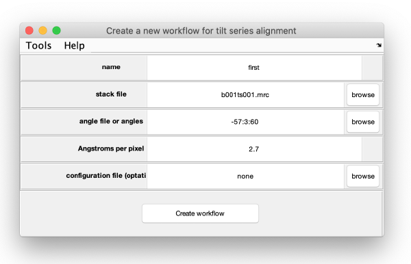
Creating an alignment workflow
The basic function for invoking the GUI is dtsa (short form of dynamo_tilt_series_alignment;
u = dtsa();
Here, u is an object that will reside in memory during the session and allows to interoperate with the workflow through the command line. It is not necessary when proceeding through the GUI.
The data for the workflow (tilt series, angles) could have been introduced directly when creating the workflow, we however will introduce each item explicitly in this walkthrough.
The minimal data to initiate a workflow is
- tilt series matrix (use the file indicated above)
- tilt angles.
- discarded tilt angles (leave empty)
Discarded tilt angles
If you are unsure on the tilts to be discarded, you can do it in a later stage while you inspect the images in the dmarkers GUI, using the x and shift + x buttons.
GUI description
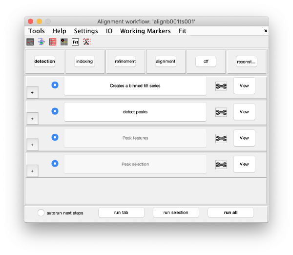
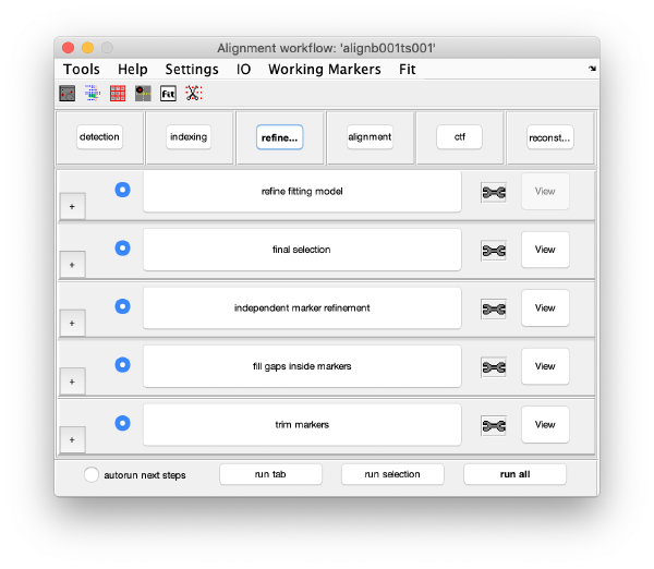
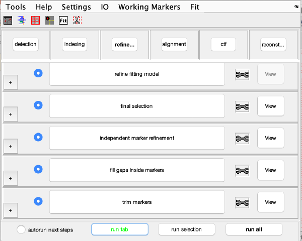
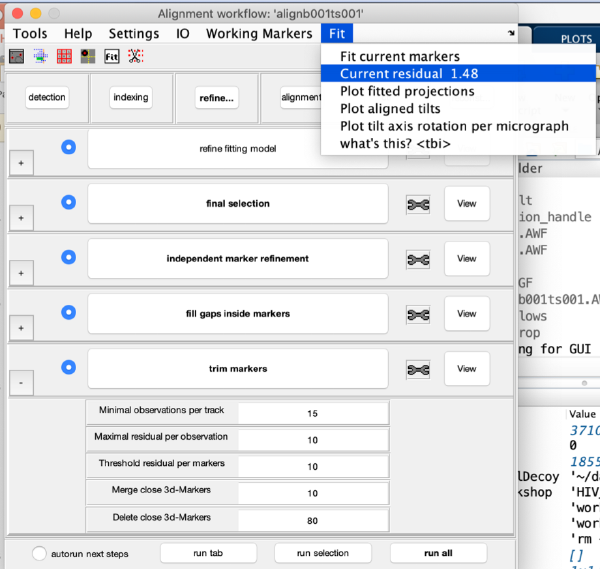
The GUI guides of the process of creating and editing a set of "working markers" (in the areas of detection, reindexing and refinement), and then using them to create aligned stacks (alignment tab), analyse and correct their CTF (through wrappers to ctfffind4 and imod) and then create reconstructions.
Settings
Acquisition settings
Here you can enter pixel size (2.7 Angstroms), Cs (2.2), nominal defocus (-4.0 microns, used if the CTF area is connected).
Controls
markers GUI
The icon of the markers GUI allows you to check the position of the working markers in the micrograph. If you want to make editions of the GUI permanent, you need to save the current markers.
Occupancy plot
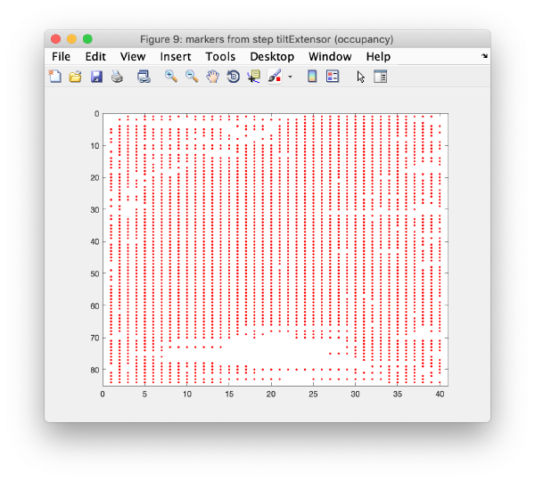
Shows a scheme of which markers are present in which tilt numbers.
Gold bead gallery
Crops the gold beads currently contained in the working markers and shows them as a gallery.
Execution Areas
The GUI is divided in five areas. Each are comprises sets of steps that can be executed sequentially. Sequential execution is the natural way of proceeding; but steps can be visited in any order, i.e., a step can be reexecuted in a later moment after updating its information.
Steps
Steps needs to be open (letters in black, not grey) in order to be executed. They become open when the input they require gets computed and stored by a previous step during execution of the workflow. When a step is under execution, its pushbutton becomes green.
Step Toolbox
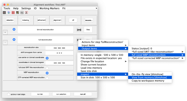
The tool icon can be secondary clicked and will provide a popup menu with specific tools for each steps and some common one. The common ones are handles to inspect and list the items that are needed (input items) or generated (output items) by the step. The View provides tools specific for visualisation of results of the step.
The areas in the alignment task
Detection
The goal of this task is to find the positions of the gold bead projections in the tilt series.
Visualization matrix
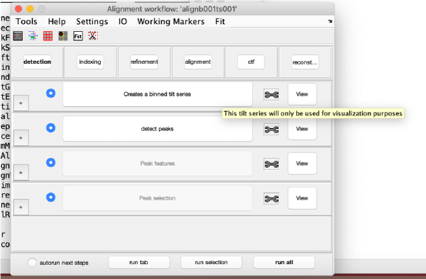
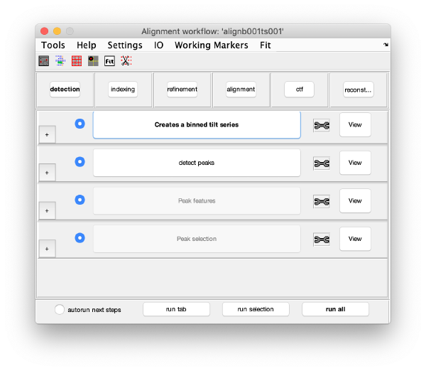
This step just creates a binned version of the tilt series stack to accelerate visualizations that will be invoked in a later point.
Detection of gold beads
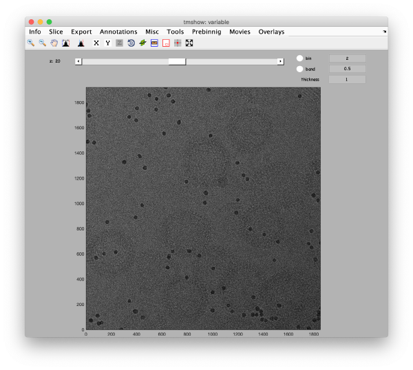
This area is the one that needed some design decision on the size of the gold bead. We will use dtmshow
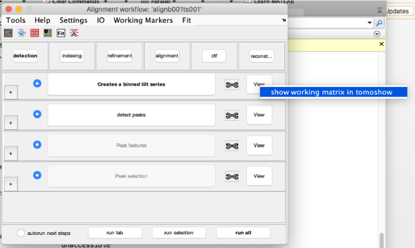
Right click on the view area of the step to access the different visualisation options.
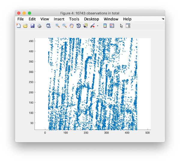
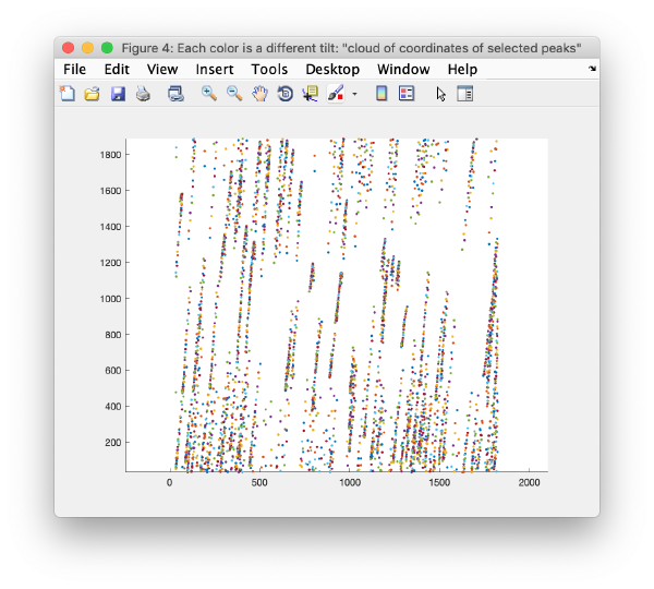
This view shows the x,y coordinates of all cross correlation peaks on all the micrographs in the tilt series.
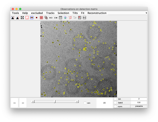
We can also check the positions of all the detected spots on each micrograph:
This GUI does not allow for edition of the markers.
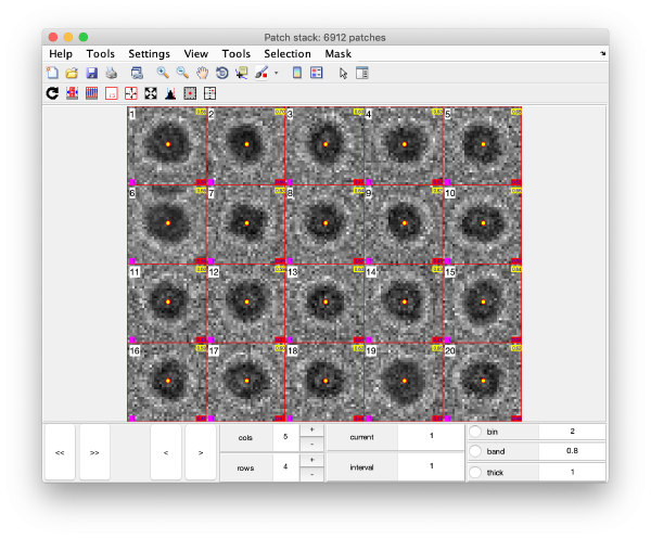
The neighbourhood of cross correlation peaks can be visualised individually:
This visualization is normally a good gauge on how the detection procedure has worked. The example below would be an example of detection procedure carried with wrong search parameters
Note that you have the option of testing your parameters against a single image before launching a full detection procedure.
Computation of observation features s
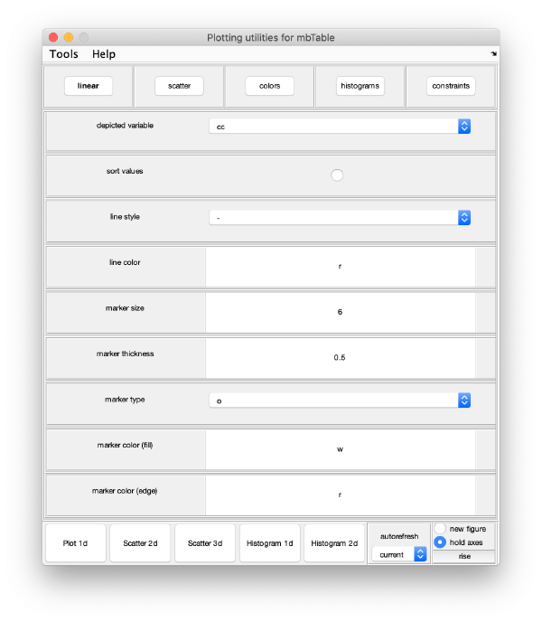
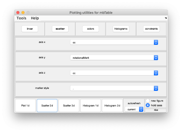
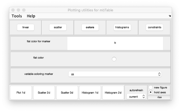
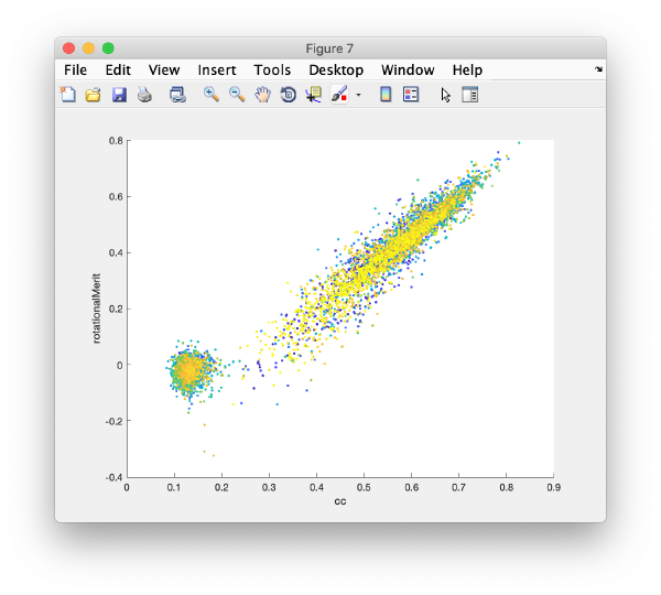
At this stage, the observed cross correlation peaks are analysed. In the current Dynamo' version a merit figure is assigned to each peak based on a "rotational merit" that measures its similarity to a circle. The results can be depicted on patches representing individual gold beads:
or extracting properties of the whole data set.
Selection of best gold beads
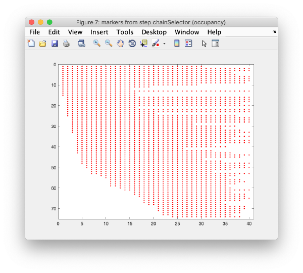
The cluster with the best markers is then selected. The individual patches can be inspected
or, again the cloud of observations
and the location of the observations in the micrographs:
Indexing
The goal of this task is to find trails of gold beads, i.e., observations in different micrographs that correspond to the same 3d gold bead.
Rough Alignment
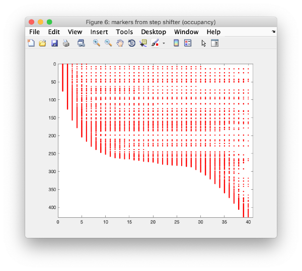
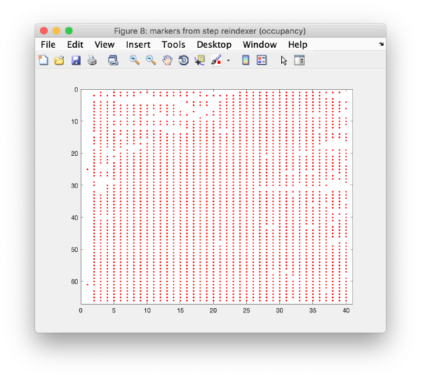
Here all couples of micrographs are compared. For each couple, we look for the relative shifts that generates the most matches of cross-correlation peaks between one micrograph and the next one. This procedure induces trails of matched pairs of observations of variable length along the tilt series. The scheme that depicts which trails have representatives in which tilts is called occupancy graph
Note that these trails are very lacunary and don't conserve the identity of a trail; whenever a trail that represents an actual 3d marker gets interrupted, the same 3d marker might generate a different trail in other tilts.
Selection of stable trails
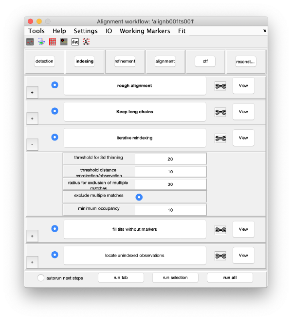
Iterative reindexing
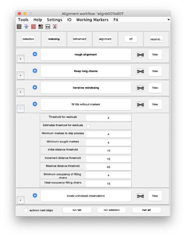
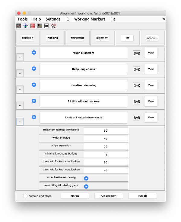
Tilt gap filling
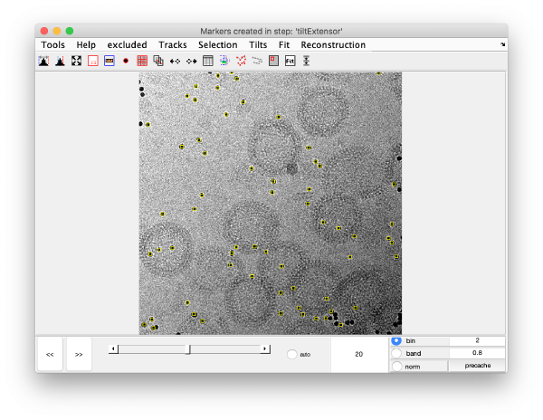
Trail extension
Refinement
Alignment
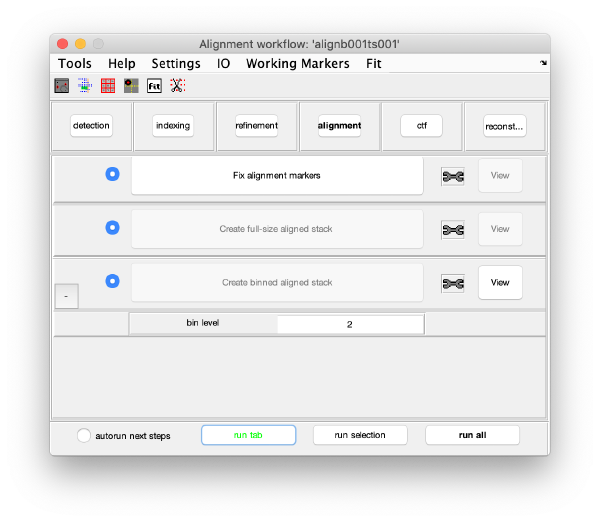
This area creates the aligned tilt series.
Fix the markers
Align the tilt series
CTF
In this GUI CTF estimation and correction are delegated to CTFFIND4 and Imod's ctfphaseflip programs respectively. This part will not be used in the workshop.'
Reconstruction
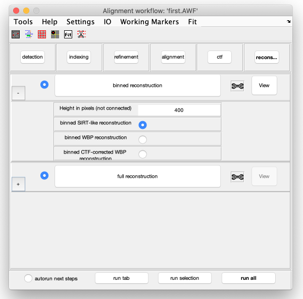
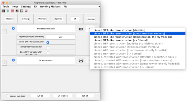
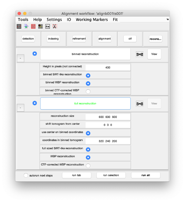
Binned reconstruction
Full sized reconstruction
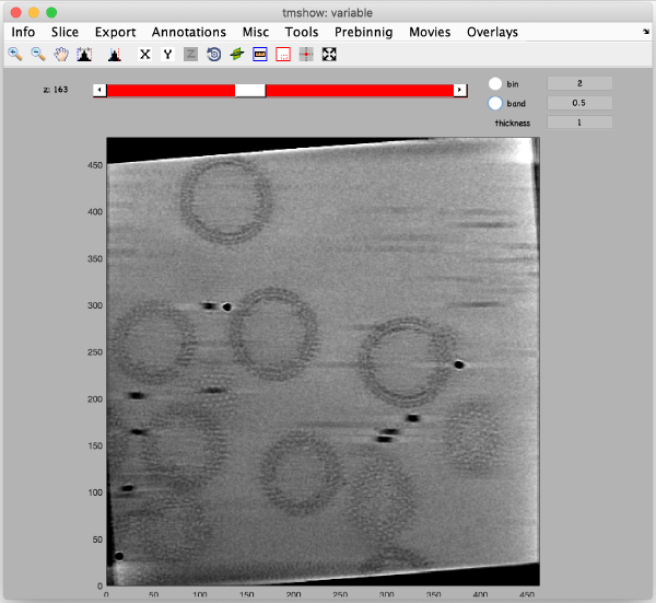
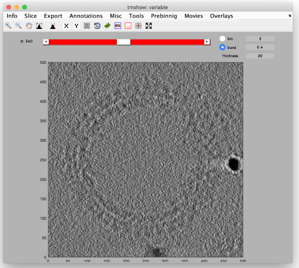
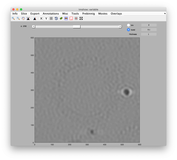
The full sized reconstruction can be created related to a coordinate directly read in the binned tomogram, a feature useful for creating reconstructions localised on an area of interest. In this case, we will focus on one of the VLPS.
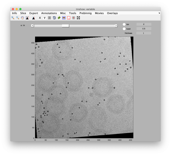
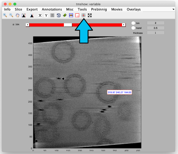
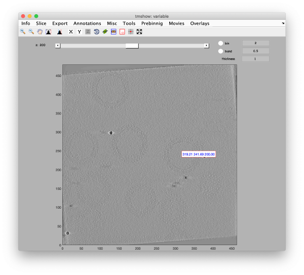
Use the pin tool to select a point on the binned reconstruction.
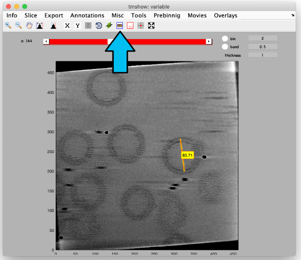
We also check the size of a structure of interest. We measure it in the binned tomogram.
]

