Difference between revisions of "Example of use of dcoordinates"
| (One intermediate revision by the same user not shown) | |||
| Line 1: | Line 1: | ||
| − | This is a toy example to illustrate the conversion of volumes into spherical coordinates through the command <tt>dcoordinates</tt>. | + | This is a toy example to illustrate the conversion of volumes into spherical coordinates through the command <tt>dcoordinates</tt>. This function has not been optimized (is purely written in Matlab, without a C++ core), and will probably stuck your computer for volumes with a size above 256 pixels of sidelength. |
| − | We will create a small virus model by attaching a regular distribution of ''spikes'' (cylinders) to a virus (a sphere) | + | We will create a small virus model by attaching a regular distribution of ''spikes'' (cylinders) to a virus (a sphere with a radius of 30 pixels): |
<pre>vol = dsphere(30,256); | <pre>vol = dsphere(30,256); | ||
| Line 22: | Line 22: | ||
Remember that <tt>disoview</tt> is a very basic renderer of isosurfaces. We use it as a fallback when Chimera is not performing in the system. | Remember that <tt>disoview</tt> is a very basic renderer of isosurfaces. We use it as a fallback when Chimera is not performing in the system. | ||
| − | [[File: | + | [[File:MercatorIsosurface.png|center|right|400px| <tt>disoview</tt> ]] |
| − | Alternatively we can visualize the grey map | + | Alternatively we can visualize the grey map: |
| − | [[File: | + | [[File:MercatorDview.png|center|right|400px| <tt>dview</tt> ]] |
Now we can perform the coordinate conversion: | Now we can perform the coordinate conversion: | ||
| Line 39: | Line 39: | ||
dshow(squeeze(sum(vols(28:32,:,:),1))); </pre> | dshow(squeeze(sum(vols(28:32,:,:),1))); </pre> | ||
| − | [[File: | + | [[File:MercatorRadiusClose.png|centering|center|400px| <tt>dshow</tt> of surface of virus ]] |
Here, | Here, | ||
| Line 50: | Line 50: | ||
dshow(squeeze(sum(vols(35:40,:,:),1)));</pre> | dshow(squeeze(sum(vols(35:40,:,:),1)));</pre> | ||
| − | [[File: | + | [[File:MercatorRadiusFar.png|center|right|400px| <tt>dshow</tt> of spikes far away from radius of virus ]] |
Latest revision as of 18:44, 12 February 2019
This is a toy example to illustrate the conversion of volumes into spherical coordinates through the command dcoordinates. This function has not been optimized (is purely written in Matlab, without a C++ core), and will probably stuck your computer for volumes with a size above 256 pixels of sidelength.
We will create a small virus model by attaching a regular distribution of spikes (cylinders) to a virus (a sphere with a radius of 30 pixels):
vol  = dsphere(30,256);
v = dmodels.vesicle();
v.center = 128.5*[1,1,1];
v.separation = 20;
v.radius = 40;
v.updateCrop;
t = v.grepTable();
myTemplate = dcylinder([4,12],24);
mask      = myTemplate;
for i=1:size(t,1);
   rotTemplate = dynamo_rot(myTemplate,t(i,7:9));
   rotMask     = dynamo_rot(mask,t(i,7:9));
   vol = dpkvol.embed(rotTemplate,vol,t(i,24:26),rotMask);
end
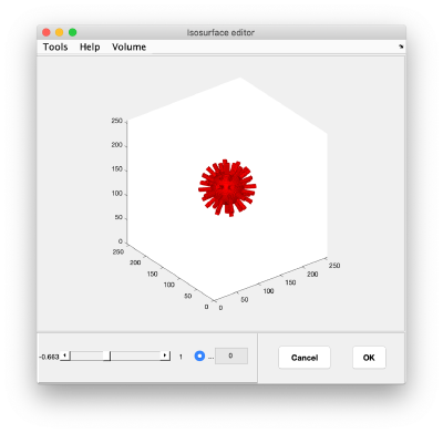
We can quickly check how our "virus" looks like:
disoview(vol);
Remember that disoview is a very basic renderer of isosurfaces. We use it as a fallback when Chimera is not performing in the system.
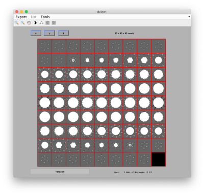
Alternatively we can visualize the grey map:
Now we can perform the coordinate conversion:
vols = dcoordinates(vol,'cart2sph');
After this transform, the radial direction is stored along the first dimension of vols. Second and third dimension correspond to the spherical angles.
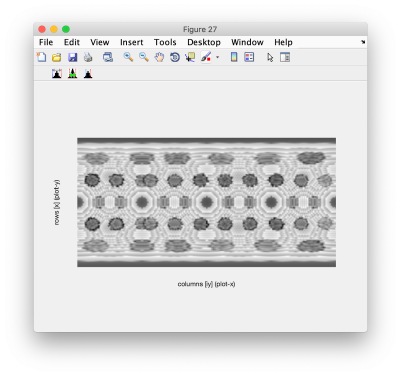
We can now check the surface of the virus at the radial distance 30 (the "surface" of the virus in this example), adding layers 28 to 32.
figure;
dshow(squeeze(sum(vols(28:32,:,:),1)));
Here,
- vols(28:32,:,:); corresponds to extracting the layers 28 to 32 in the volume vols
- the sum command adds all the layers of the argument along the direction 1 (the radial direction in this case)
- the squeeze command is just Matlab formating: it converts the (nominal) volume created by sum (with dimensions 1 x 256 x512) into an image 256 x 512 that can then be fed into show;
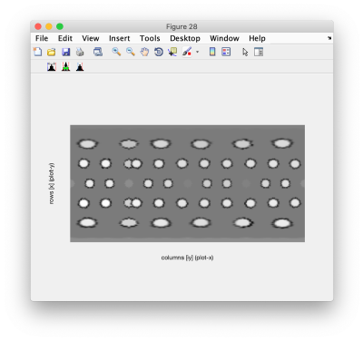
A clearer view can be gained by averaging some pixels away from the surface:
figure;
dshow(squeeze(sum(vols(35:40,:,:),1)));


