Difference between revisions of "Walkthrough for template matching"
| Line 58: | Line 58: | ||
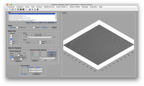
We use for this our tool <tt>dtmslice</tt>. As the tomogram is provided is fairly small you can probably just open it without any further binning. | We use for this our tool <tt>dtmslice</tt>. As the tomogram is provided is fairly small you can probably just open it without any further binning. | ||
| − | <tt>dtmslice t20s.mrc - | + | <tt>dtmslice t20s.mrc -c ct20</tt> |
[[ File:TemplateMatchingTomosliceGeneral.png |thumb|center|500px| <tt>dtmslice</tt> on tomogram ]] | [[ File:TemplateMatchingTomosliceGeneral.png |thumb|center|500px| <tt>dtmslice</tt> on tomogram ]] | ||
Revision as of 20:33, 21 August 2017
Dynamo includes a set of tools for location of particles inside tomograms. The most simple one is template matching.
Contents
Template matching
In this technique, a template representing a molecule of interest is systematically cross-correlated against a tomogram, producing a cross-correlation map of the tomogram. Each pixel in this map represents a score assigned the corresponding pixel in the tomogram map. This score measures the similarity of the neighbourhood of the tomogram pixel to the used template. This similarity is measured exclusively inside a mask.
Data set
Tomogram description
The tomogram contains a buffer with T20S proteasome on a holey carbon grid collected on a Krios + K2. Original pixelsize was 1.76 angstroms. The tomogram provided here has bin binned twice (yielding thus 7.04 ang), defocus is 4.4 microns, no CTF correction, no energy filter.
Acknowledgements
The tomogram has been kindly provided by Alex Noble, from the New York Structural Biology Center. Data collection was performed using Leginon and Appion-Protomo at the Simons Electron Microscopy Center and National Resource for Automated Molecular Microscopy located at the New York Structural Biology Center, supported by grants from the Simons Foundation (349247), NYSTAR, and the NIH National Institute of General Medical Sciences (GM103310) with additional support from Agouron Institute [Grant Number: F00316].
Getting the tomogram
In Linux, you can write:
wget https://wiki.dynamo.biozentrum.unibas.ch/w/doc/data/t20s/t20s.mrc
the corresponding command is curl -O in the Mac.
Visualizing the tomogram
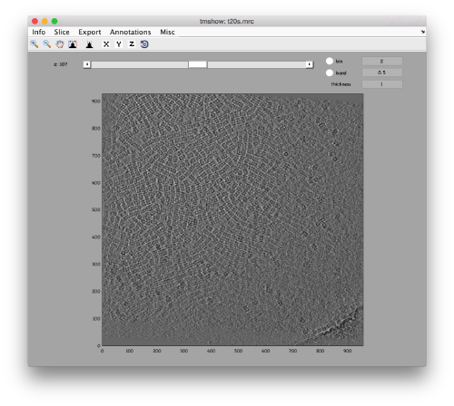
We can get a first glance on how the tomogram looks like:
dtmshow -otf t20s.mrc
to use the on-the-fly access to the slice shown at each given moment, or
v = dread('t20s.mrc');dtmshow(v);
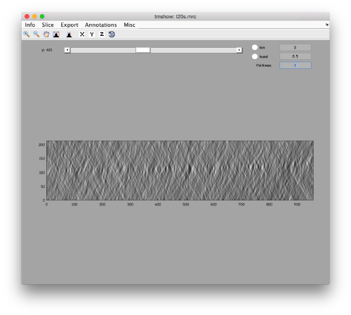
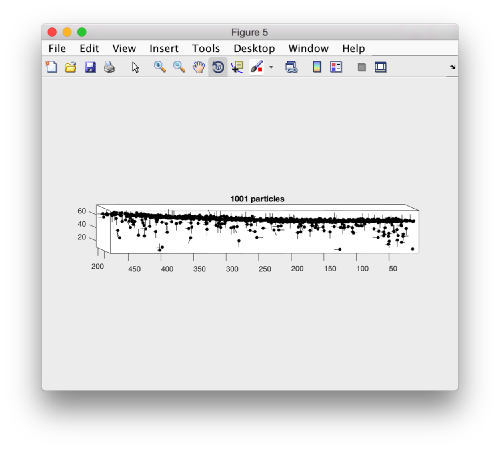
to preload the full tomogram into a memory variable (arbitrarily called v). In either option, you will see, the proteasomes are densely packed in an layer. The layer is slightly oblique, what can be seen browsing through z or y.
Navigating on-the-fly you'll see that transitions in y are slower than transitions in z, because all the pixels of the same slice are stored sequentially in the disk.
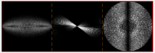
Estimation of the missing wedge
Creating a template
There are different strategies to create the first template. In the case where the general shape of each protein is roughly recognisable by eye, it is not difficult to just crop and align manually some of the particles. When this is not possible, you have the option of using a density map that mimics the general topology of your protein.
Through manual alignment
We will use a model inside tmslice to pick a set of ~10 particles. We will then crop them, and align them manually using dgallery
Manual selection of some particles
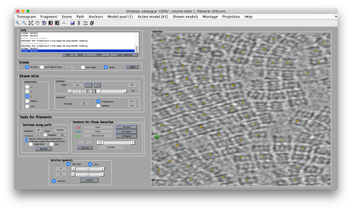
We use for this our tool dtmslice. As the tomogram is provided is fairly small you can probably just open it without any further binning.
dtmslice t20s.mrc -c ct20
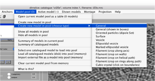
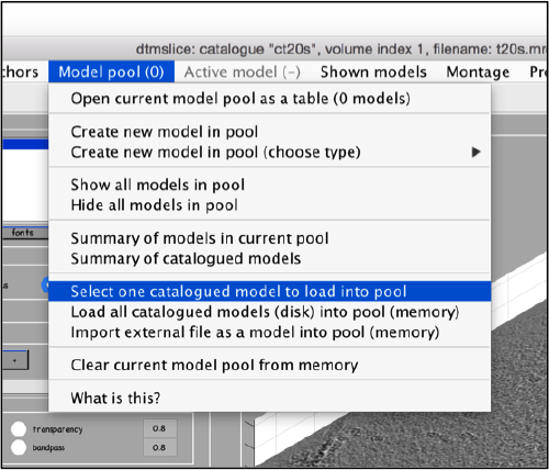
Use the model pool menu to add a new model of type General
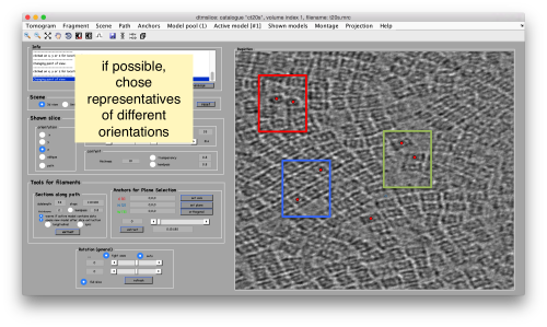
Try to pick particles on different orientations, both in top and side views. Particles are picked with the key C, use backspace to clear the latest selection.
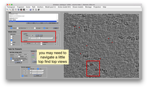
You can move the slice with the z slidebar in the control panel, or dragging it while the mouse button is pressed. Top views are more abundant below the crowded accumulation of side views in the central slice.
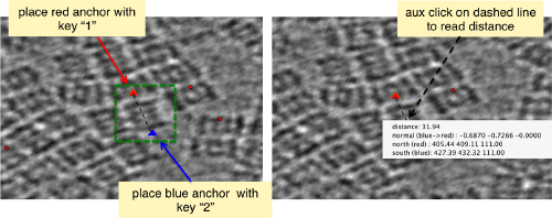
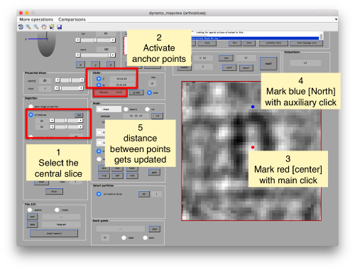
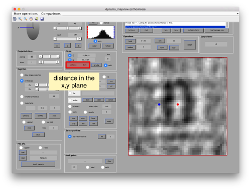
When you have clicked around ten, we will prepare to crop them out of the tomogram. For this, we need to get first an idea of how big should the box. With the keys [1] and [2] you can place anchor points in the scene. Auxiliary click in the bar between them shows the distance (in pixels of the unbinned tomogram).
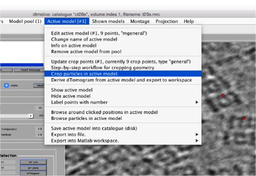
Now we can open the dtcrop utility for this model, by visiting the Active model" menu.
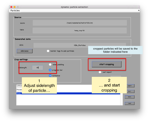
In the GUI that pops up we can fix the sidelength.
After completion of the cropping process, you will get a data folder called t20s_Particles, which will also contain a table file called t20s_Particles/crop.tbl
Manual alignment of some particles
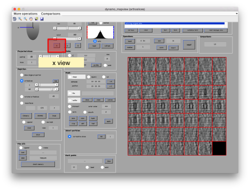
Now we want to align the particles. We open them inside the dgallery browser:
dgallery -d t20s_Particles -t t20s_particles/crop.tbl
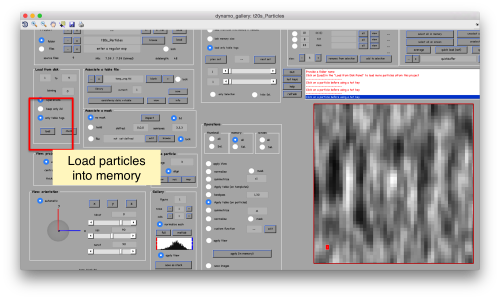
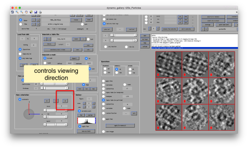
This GUI has several functionalities. We will focus in using it to quickly get an alignment of the particles. For this, we first load the particles expressed in the table into the internal memory of the gallery by clicking into Load.
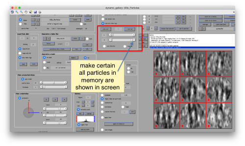
This seems not to have any effect in the depiction: you need to fix the range of the depicted particles moving the slider bar. When you do so, each particle will appear in the scene as a single red box.
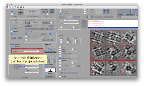
You can play with different settings for viewing, like the direction (x, y or z)
or the number of slices that are projected into the depicted image for each particle.
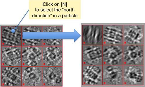
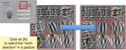
Then, you go through each particle and indicate a point that you considere that could lay in the central axis of the particle by clicking on N. The particle will rotate on screen to match this direction. The center of the particle can also be set by clicking on N
You may need to complete two rounds of operating on the particles, changing the viewing direction (first in x, then in y)
Averaging manually aligned particles
We export the table we have computed and use it to create and average
o = daverage('t20s_Particles','t','quickbuffer.tbl');
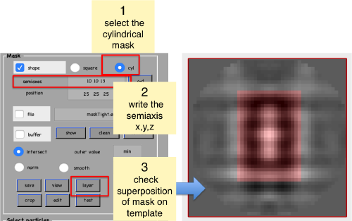
Creating a tight mask
Measure distances
Open the computed average in mapview,
dmapview(oa.average);
set the view to the XZ or YZ planes, connect the anchors [C] and [N] (which in mapview are placed simply with the main and the auxiliar click), and measure the semiaxis of the average:
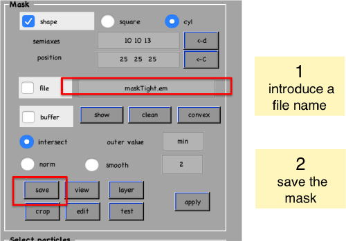
Create mask
Cropping the borders of a template
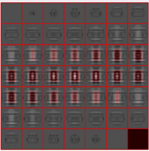
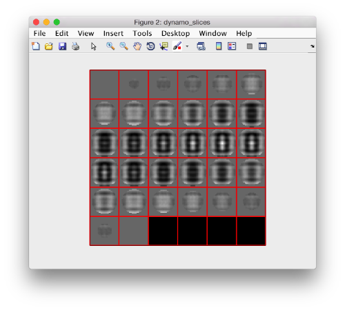
shifted =circshift(dsym(o.average,'c17'),[0,0,-1]);dslices(final,'y','overlay','maskTight.em','overlay_as','mask');
and we can actually extract the part of the template volume where we actually have signal.
cropped = dynamo_crop(shifted ,32);
Through geometrical shapes
Alternatively, you can use dynamo_mask or dynamo_tube to create a synthetic model.
Creating a template matching process
The main function is dynamo_match
pts = dynamo_match(fileFull,'average32.em','mask','maskData32.em',....
    'outputFolder','cs30',...
    'ytilt',[-39,36],'sc',[256,256,256],'cr',360,'cs',30,'bin',1);
- 'bin'
allows binning on the fly. Template, mask and tomograms are input in original size. - 'sc' : size of chunk
This is the maximum extent of a block in the unbinned tomogram that will be kept in memory by each one of the processors working in parallel (only one in this experiment). We need to be careful not to crowd the available memory. - 'cr' : cone range
orientations will be looked for inside a cone. In this context, the most usual values are 360 (sample the full sphere) or 0 (do not scan orientations)
You should get the following response on the screen (will take around 5 minutes to complete)
------------------------------------------------------------

 Template matching process.
 computing in CPU
 Output folder: cs30.TM
A total of 1 tiles have been created
  - Mb per tile (reading)   : 724.19
  - Mb per tile (operation) : 663.84
 ... initializing output elements
Preparing to run on 25 blocks
Running on single processor
 Computing tile 1

  <Information for each block>

  ... tile 1 finished in 387 seconds (8 for setup;  7.73 per triplet)
  [ok] ... template matching process completed upto creation of cross correlation
       you can proceed to peak location and particle extraction.
------------------------------------------------------------
The main result of dynamo_match is a volume (cross correlation volume) that assigns a score to each pixel. This tomogram is written in the file cs30/CC.mrc. Some auxiliary outputs are other volumes that store the angles [tdrot,tilt,narot] that maximize the cross-correlation for each pixel in the volume.
The Process object
The return of the function <notwiki>ptm</nowiki> is an object that keeps track of the location of all the created output, and is used in the subsequent steps that extract the actual location of the peaks
Locating cross correlation peaks
Looking at the cross correlation map
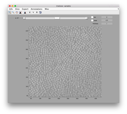
pts.showCC
Looking at the cross correlation profile
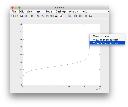
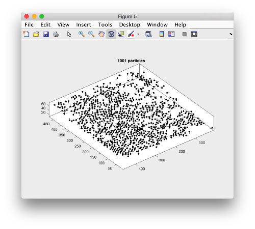
We can get a plot of the cross-correlation value found on the local maxima of the cc volume wiith the order
pts.peaks.plotCCPeaks('sidelength',32)
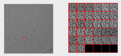
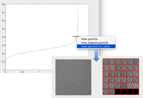
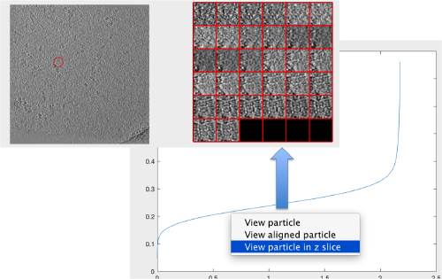
The cross-correlation values of the peaks appear in ascending order. We can check the quality of the peaks by auxiliary clicking on the curve to select one particle and then selecting some visualization option.
The sidelength that we pass will be used for this visualization options to crop the particle around the peak.
We click on a couple of particles in the area of kink in the cross-correlation to roughly estimate the cross-correlation threshold. In out case, it seems to be around 0.37 (being rather conservative)
In the gaussian distribution below this ara , the peaks do not correspond to particles
Extracting a table
A table can be extracted through:
myTable = pff.peaks.computeTable('mcc',0.378);
Visual evaluation of results
Looking at table positions
Looking at cropped particles
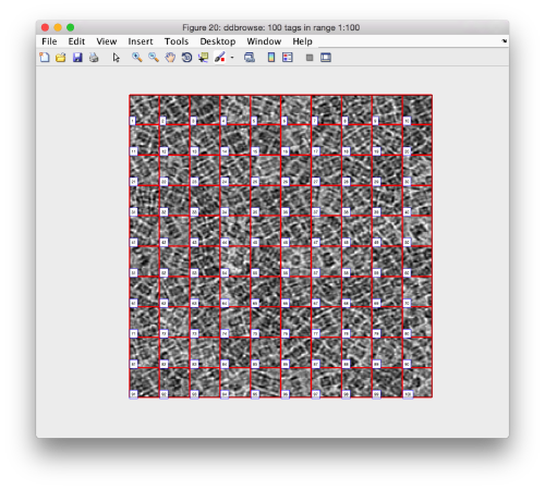
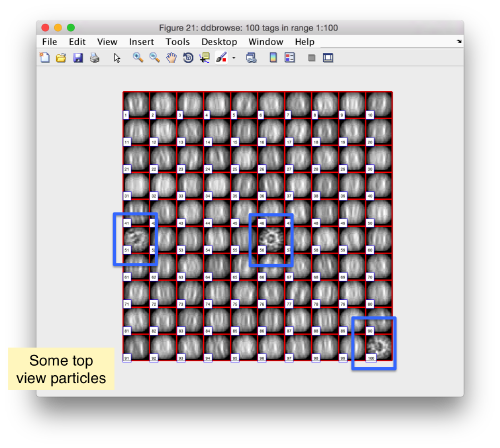
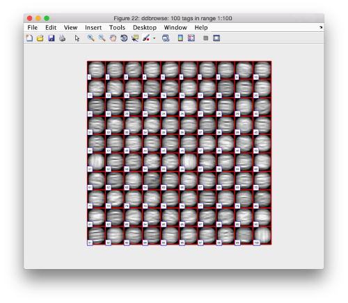
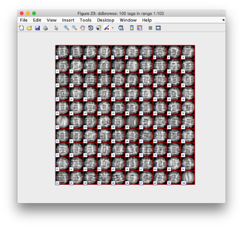
We can check how the individual particles look like on a gallery modus:
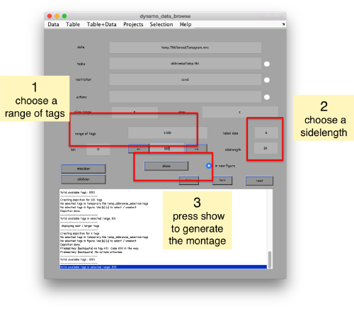
pr.peaks.browse();
This order just opens ddbrowse. We are using here the support object peaks, but this command is equivalent to just invoking ddbrowse
ddbrowse('d','cr30.TM','t',myTable);
Looking at averages
o = pff.peaks.average();
Getting the tables back into the catalogue
You don't need to operate with the catalogue: you could just use dtcrop on the just computed table to extract particles from the original tomogram into a data folder. However, cataloguing has to advantages:
- Eases keeping track of all the steps you've performed, specially if you are going to use several tomograms, and..
- allows you to visualize the peaks on the tomogram interactively, so that you can delete false positives or add peaks that were not located by the template matching.
Rescaling the table
Remember that the table that we are working with has the scale of the auxiliary binned volume that has been created along with the CC matrix. In the catalogue, we want to work with the particles in their original scale.
tableOriginalScale = dynamo_table_rescale(myTable,'factor',2);
In the syntax of dynamo_table_rescale, the factor is expressed in terms of how many times is the apix in the original table bigger than in the target table to be computed. In our case, the target table was computed with an apix of 14 Angstrom (one time binned in relation to the tomogram t20s.rec, with an apix of 7.04A). The factor is thus 2. In case of doubt, it is convenient to just run
dtinfo(tableOriginalScale);
to check the extent of the entries in the columns 24, 25 and 26, which are positions (in pixels) of the particles indexed by the table. Now, if we write the upscaled table into a file
dwrite(tableOriginalScale,'peaks.tbl');
we can just put this table back into the catalogue through:
dmimport -t peaks.tbl -c ct20s -i 1 -mn ccpeaks
which will create a model called ccpeaks and assign it to the first volume (-i 1) in the catalogue ct20s. You can check it by writing:
dcm -c ct20s -i 1 -l m
which asks for a listing of models (-l m) in the first volume of the catalogue.
