Difference between revisions of "Starters guide"
| (23 intermediate revisions by 4 users not shown) | |||
| Line 8: | Line 8: | ||
* Avoiding overfitting via independent half dataset refinement (“gold standard processing”) | * Avoiding overfitting via independent half dataset refinement (“gold standard processing”) | ||
| − | + | Streamlined workshop version of this tutorial: [[Starters_guide_(workshop_version)| here]]. | |
==Introduction== | ==Introduction== | ||
| Line 16: | Line 16: | ||
[[Downloads|Download]] ''Dynamo'' and copy the .tar file to your desired [[installation]] directory <tt><DYNAMO_ROOT></tt> and untar it: | [[Downloads|Download]] ''Dynamo'' and copy the .tar file to your desired [[installation]] directory <tt><DYNAMO_ROOT></tt> and untar it: | ||
| − | <tt>tar -xvf dynamo-v-1.1.50_MCR-8.2.0_GLNXA64.tar </tt> | + | <tt>tar -xvf dynamo-v-1.1.50_MCR-8.2.0_GLNXA64.tar </tt> |
(for Linux and Mac systems or use a visual tool as 7-zip under Windows) | (for Linux and Mac systems or use a visual tool as 7-zip under Windows) | ||
| Line 25: | Line 25: | ||
Start Matlab in your system (can take some time), an inside the Matlab terminal, type | Start Matlab in your system (can take some time), an inside the Matlab terminal, type | ||
| − | <tt>>> run <DYNAMO_ROOT>/dynamo_activate.m</tt> | + | <tt>>> run <DYNAMO_ROOT>/dynamo_activate.m</tt> |
Dynamo is now ready to use. Make a new directory for your project (>> mkdir dtutorial) and go there | Dynamo is now ready to use. Make a new directory for your project (>> mkdir dtutorial) and go there | ||
| Line 33: | Line 33: | ||
''Dynamo'' has a help center that may be called by typing | ''Dynamo'' has a help center that may be called by typing | ||
| − | <tt>>> dhelp</tt> | + | <tt>>> dhelp</tt> |
It contains descriptions for all the dynamo functions that may be also called from the Matlab command line with customized parameters. You can also type >> help dynamo_function_name for the lists of parameters for each function. Help center also contains descriptions of data types (list of database items). Finally you can view a list of PDF tutorials with examples that demonstrate advanced usage of ''Dynamo''. Note that simple copy-pasting of some commands from PDF into Matlab may not work under Linux due to special characters. Another way to access documentation is to ask ''Dynamo'' about it. Type >> dapropos to get the list of potential entries for the subject. You can use it without parameters get the list of topics or ask about a particular topic like >> dapropos table. More advanced users can use >>dlookfor to find functions containing a given string in their name or code. | It contains descriptions for all the dynamo functions that may be also called from the Matlab command line with customized parameters. You can also type >> help dynamo_function_name for the lists of parameters for each function. Help center also contains descriptions of data types (list of database items). Finally you can view a list of PDF tutorials with examples that demonstrate advanced usage of ''Dynamo''. Note that simple copy-pasting of some commands from PDF into Matlab may not work under Linux due to special characters. Another way to access documentation is to ask ''Dynamo'' about it. Type >> dapropos to get the list of potential entries for the subject. You can use it without parameters get the list of topics or ask about a particular topic like >> dapropos table. More advanced users can use >>dlookfor to find functions containing a given string in their name or code. | ||
| Line 40: | Line 40: | ||
In a Linux/Mac shell, type: | In a Linux/Mac shell, type: | ||
| − | <tt>>> source <DYNAMO_ROOT>/dynamo_activate_linux_shippedMCR.sh</tt> | + | <tt>>> source <DYNAMO_ROOT>/dynamo_activate_linux_shippedMCR.sh</tt> |
==Particle picking and ''Dynamo'' catalogues== | ==Particle picking and ''Dynamo'' catalogues== | ||
| − | We assume that your tomograms are already generated using external packages (i.e. IMOD, Protomo, Inspect3D, TOM); for this tutorial ''Dynamo'' will generate simulated data. The ''Dynamo'' catalogues are databases that manage tomograms and link the tomographic data to the extracted particles. Start catalogue manager from the ''Dynamo'' command window. | + | We assume that your tomograms are already generated using external packages (i.e. IMOD, Protomo, Inspect3D, TOM); for this tutorial ''Dynamo'' will generate simulated data. The ''Dynamo'' catalogues are databases that manage tomograms and link the tomographic data to the extracted particles. Start [[catalogue manager|Dcm GUI ]] from the ''Dynamo'' command window. |
| + | |||
| + | <tt>dcm</tt> | ||
| + | |||
| + | This command will work equally in Matlab and in the standalone, producing the [[Dcm GUI]]. Once it opens, in the catalogue manager window use menu ''Help -> Create synthetic examples -> Create a synthetic catalogue''. | ||
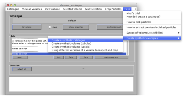
[[File:StartersGuideFigure1.png|thumb|center|600px| Figure 1: creating a set of synthetic tomograms with ''Dynamo'' Catalogue Manager]] | [[File:StartersGuideFigure1.png|thumb|center|600px| Figure 1: creating a set of synthetic tomograms with ''Dynamo'' Catalogue Manager]] | ||
| Line 51: | Line 55: | ||
===Viewing tomograms=== | ===Viewing tomograms=== | ||
You can see the list of your tomograms and metadata in a table in the bottom of your [[dcm | catalogue manager window]]. You can add tomograms to the catalogue by ''Catalogue -> Browse for new volume''. You can get an overview of your tomograms in the catalogue by ''View all volumes -> create thumbnails'' and ''View all volumes -> show thumbnail gallery''. All these functionalities have their corresponding command line versions, accessible through the <tt>dcm</tt> command (short for <tt>dynamo_catalogue_manager</tt>), whose options and syntax can be consulted through <tt>>> doc dcm</tt>. | You can see the list of your tomograms and metadata in a table in the bottom of your [[dcm | catalogue manager window]]. You can add tomograms to the catalogue by ''Catalogue -> Browse for new volume''. You can get an overview of your tomograms in the catalogue by ''View all volumes -> create thumbnails'' and ''View all volumes -> show thumbnail gallery''. All these functionalities have their corresponding command line versions, accessible through the <tt>dcm</tt> command (short for <tt>dynamo_catalogue_manager</tt>), whose options and syntax can be consulted through <tt>>> doc dcm</tt>. | ||
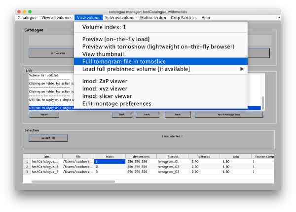
| − | ''Dynamo'' has several viewers designed for various purposes. Select the first tomogram in the list with a mouse click and go to ''View volume | + | ''Dynamo'' has several viewers designed for various purposes. Select the first tomogram in the list with a secondary mouse click and go to ''View volume>Full tomogram file in tomoslice'' . |
| − | [[File: | + | [[ File:StartersSelectTomoSliceInCatalogue.png |thumb| center |600px| Figure 2: Selecting a volume in the catalogue manager to be inspected in <tt>dpreview</tt>]] |
| − | [[ | + | The volume browser [[dtmslice | tomoslicer]] loads the entire tomograms into memory and allow making annotations to the regions of interest. The tomograms in this tutorial are small, and you can load them directly into memory. For real life tomograms, bear in mind that you will need to [[Prebinned tomograms| prebin]] the files before loading them into memory (or alternatively, load fragments of them using <tt>dpreview</tt>) |
| − | + | Tomoslice has a simple set of controls, and is suitable for visualization tasks that require oblique sections through the tomogram. It uses the same tool as other ''Dynamo'' browsers to keep track of your annotations: a pool of models. | |
Go to ''View volume -> load full tomogram into Tomoslice''. On the left control panels Scene turn off the 3d view radiobutton. You can navigate the z-height of the tomogram with a mouse wheel or with a slider in the tomoslice menu (1 to 256 in this case); you can also change the slice thickness from the default 10 pixels. Play with the controls and explore the tomogram. Turn 3d view back on. | Go to ''View volume -> load full tomogram into Tomoslice''. On the left control panels Scene turn off the 3d view radiobutton. You can navigate the z-height of the tomogram with a mouse wheel or with a slider in the tomoslice menu (1 to 256 in this case); you can also change the slice thickness from the default 10 pixels. Play with the controls and explore the tomogram. Turn 3d view back on. | ||
| Line 100: | Line 104: | ||
[[File:StartersGuideParticlesUnaligned.png|thumb|center|400px| Particles without alignment (<tt>table</tt> is switched off).]] | [[File:StartersGuideParticlesUnaligned.png|thumb|center|400px| Particles without alignment (<tt>table</tt> is switched off).]] | ||
 |  | ||
| − | |||
==Subtomogram alignment and averaging== | ==Subtomogram alignment and averaging== | ||
===Initial model generation=== | ===Initial model generation=== | ||
| − | If you don’t have an initial model it is easy to generate it by manually aligning several particles and summing them up. ''Dynamo'' stores information about the particles in dynamo tables: for each particle a table contains shifts and rotations to bring the particle to the average (by default these values are initialized as 0s), particle ID (tag), orientation of the missing wedge and others. For full info type <tt>>> dthelp</tt> in Matlab. ''Dynamo'' catalogue generates an initial table during particle extraction, its location is particles/crop.tbl | + | If you don’t have an initial model it is easy to generate it by manually aligning several particles and summing them up. ''Dynamo'' stores information about the particles in dynamo tables: for each particle a table contains shifts and rotations to bring the particle to the average (by default these values are initialized as 0s), particle ID (tag), orientation of the missing wedge and others. For full info type <tt>>> dthelp</tt> in Matlab. ''Dynamo'' catalogue generates an initial table during particle extraction, its location is <tt>particles/crop.tbl </tt> |
| + | |||
| + | ==== Loading particle in <tt>dgallery</tt> ==== | ||
| + | |||
| + | For initial model generation we will use dynamo_gallery to generate initial orientations for some of our particles. Type | ||
| + | |||
| + | <tt>>> dgallery(‘data’, ‘exampleData.Data’); </tt> | ||
| + | |||
| + | assuming you named <tt>exampleData</tt> your data folder while cropping. | ||
| + | |||
| + | * Load particles into memory by clicking “load” in the Load from disk field on the left of the window. Note that at first, the scene will show only '''one''' particle. | ||
| + | * Display some or all of the particles with the slider in the <tt>Shown</tt> particles field on the top of the window. | ||
| + | * Toggle between X- Y- and Z-views in the View: orientation field. | ||
| + | |||
| + | ==== Manual alignment of particles in <tt>dgallery</tt> ==== | ||
| + | |||
| + | Now for each particle you can specify the center with a mouse click and the “C” button. Thermosomes are barrel-like particles with a long axis, you therefore may also specify the “top” of the particle by clicking along the long axis of the particle (but still within the box) with a mouse click and click “N” (stands for North). Do it for all the particles alternating the X- Y- and Z- views. Non-aligned particles are marked red, once the particle has been left-clicked it adds to the section in memory and turns blue. To remove from selection right click on the box. | ||
| − | <tt | + | ==== Selecting particles in <tt>dgallery</tt> ==== |
| − | + | You can save selected tags and a corresponding dynamo table by clicking the “quick save” button in the Particle Section field on top of the window. It saves a quickbuffer.tbl and quickbuffer.tags to the hard drive that you will use later. | |
| + | |||
| + | ==== Averaging selected particles ==== | ||
To generate the average you need to “apply” the table on the particles. For this click the “average” button in the Particle selection field. It opens dynamo_average_GUI with a lot of controls, we only need output filename in the Averaged volume field - my_average.em. Click “compute average” in the bottom of the window; wait till it is done. Right click to the output filename and select the [view] simple 3d depiction of all slices option and examine it from X- Y- and Z- views. If you are not satisfied with the result close the window and refine your manual alignment / add more particles to the average. | To generate the average you need to “apply” the table on the particles. For this click the “average” button in the Particle selection field. It opens dynamo_average_GUI with a lot of controls, we only need output filename in the Averaged volume field - my_average.em. Click “compute average” in the bottom of the window; wait till it is done. Right click to the output filename and select the [view] simple 3d depiction of all slices option and examine it from X- Y- and Z- views. If you are not satisfied with the result close the window and refine your manual alignment / add more particles to the average. | ||
| Line 114: | Line 135: | ||
Iterative alignment of subtomograms to the average is performed by dynamo projects that you can run in various high-performance computational environments. To have a project you need particles, an initial reference and a table which you have already generated. Start a [[dcp GUI| WIZARD]] in the ''Dynamo'' command window or type | Iterative alignment of subtomograms to the average is performed by dynamo projects that you can run in various high-performance computational environments. To have a project you need particles, an initial reference and a table which you have already generated. Start a [[dcp GUI| WIZARD]] in the ''Dynamo'' command window or type | ||
| − | <tt>>> dcp</tt> | + | <tt>>> dcp</tt> |
in Matlab (<tt>dcp</tt> stands for ''dynamo current project''). Type a project name “drun1” and press Enter, ''Dynamo'' will generate the auxiliary files in a folder called <tt>drun1</tt>. | in Matlab (<tt>dcp</tt> stands for ''dynamo current project''). Type a project name “drun1” and press Enter, ''Dynamo'' will generate the auxiliary files in a folder called <tt>drun1</tt>. | ||
| Line 134: | Line 155: | ||
*''Symmetry'' – if you know the symmetry of your protein it will speed up the convergence and result in higher resolution. Here we don’t make any assumptions. | *''Symmetry'' – if you know the symmetry of your protein it will speed up the convergence and result in higher resolution. Here we don’t make any assumptions. | ||
*''Threshold parameters and modus'' specify which particles contribute to the average at the end of each iteration. Our typical values are [1,2] and [0.5,5]. | *''Threshold parameters and modus'' specify which particles contribute to the average at the end of each iteration. Our typical values are [1,2] and [0.5,5]. | ||
| − | |||
There are predefined parameter sets for Global and Local searches (''Predefined profiles -> Global search / Refinement''). After you set up the parameters press ''OK'' or close the window. | There are predefined parameter sets for Global and Local searches (''Predefined profiles -> Global search / Refinement''). After you set up the parameters press ''OK'' or close the window. | ||
| Line 140: | Line 160: | ||
[[File:StartersGuideFigure10.png|thumb|center|600px| Figure 10. Summary of numerical parameters used for sub tomogram averaging.]] | [[File:StartersGuideFigure10.png|thumb|center|600px| Figure 10. Summary of numerical parameters used for sub tomogram averaging.]] | ||
| − | Go to Computing environment in Wizard and select | + | Go to Computing environment in Wizard and select Matlab-CPU. Click “Info (nvidia)” it should output you a table to your Matlab window, your GPU identifiers are in the left column of the table. Put those into the GPU identifiers to the ‘identifiers” field. |
| − | + | ||
| + | ====Running the project==== | ||
| + | |||
| + | Go back to the Wizard window, click “check” and ‘unfold”, this will generate a runnable matlab script drun1.m. If you will modify your project and will want to run it again you need to re-unfold the project before each run. | ||
| + | |||
| + | * In a Matlab session you can just click on “run”. | ||
| + | * In a standalone project it's more convenient to open a new terminal, activate ''Dynamo'' on it and run the project just invoking the name of the project script that was generated by the unfolding step: | ||
| − | <tt> | + | <tt> ./drun1.exe</tt> |
| + | Open another Matlab window, activate dynamo, go to the same folder and monitor the progress of the execution by typing in >> dvstatus drun1. After several iterations you can look at intermediate results by typing: | ||
| + | |||
| + | <tt> >> ddb drun1:a –v </tt> | ||
| + | |||
or | or | ||
| − | <tt>>>ddb drun1:a:ite=* -j c10</tt> | + | <tt>>>ddb drun1:a:ite=* -j c10</tt> |
For more info on <tt>ddb</tt> type <tt> >> help ddb</tt>. In the end of your iterations you can monitor the results in the show results section of Wizard and should get something like this: | For more info on <tt>ddb</tt> type <tt> >> help ddb</tt>. In the end of your iterations you can monitor the results in the show results section of Wizard and should get something like this: | ||
| Line 157: | Line 187: | ||
First generate a dataset which has 2 populations of particles. For this, type: | First generate a dataset which has 2 populations of particles. For this, type: | ||
| − | <tt>>> dynamo_tutorial('data_classification','M',8,'N',8);</tt> | + | <tt>>> dynamo_tutorial('data_classification','M',8,'N',8);</tt> |
in your Matlab window. It generates two sets of particles, 8 particles in each and stores their real orientations in the directory <tt>data_classification</tt>. | in your Matlab window. It generates two sets of particles, 8 particles in each and stores their real orientations in the directory <tt>data_classification</tt>. | ||
===Multireference alignment=== | ===Multireference alignment=== | ||
| − | The idea behind [[Multireference Analysis|MRA]] is: iterative alignment of particles to several references and then each particle assigned to the reference where it fits the best. This way over iterative refinement similar particles will have higher correlation to similar references and will eventually group together. MRA is naturally implemented in ''Dynamo''. For classification into N classes we will need N initial references and N initially identical tables that ''Dynamo'' will generate automatically. The references should be slightly different to start particle differentiation, in ''Dynamo'' we add small amount of white noise to the overall average of all particles. | + | The idea behind [[Multireference Analysis|MRA]] is: iterative alignment of particles to several references and then each particle assigned to the reference where it fits the best. This way over iterative refinement similar particles will have higher correlation to similar references and will eventually group together. MRA is naturally implemented in ''Dynamo''. For classification into N classes we will need N initial references and N initially identical tables that ''Dynamo'' will generate automatically. The references should be slightly different to start particle differentiation, in ''Dynamo'' we add a small amount of white noise to the overall average of all particles. |
| − | Create a new project by typing “drun2” in the project name of Wizard set number of references to 2, set ''Swap particles'' on, put in the particle data. Go to “table” and type <tt>data_classification/real.tbl</tt> into the “clone this” field and press “copy”, press “OK”. Go to “template” and clone data_classification /original_template.em with addition of some extra noise with amplitude 1. Initialize masks with the defaults parameters (large button on the bottom). Go to “numerical parameters” and use Predefined profiles -> refinement. Increase angular search steps to 5, set a thresholing policy and press “OK”. Set computing environment to GPU (under Matlab), specify GPU identifiers. | + | |
| + | ==== Creating MRA projects ==== | ||
| + | Create a new project by typing “drun2” in the project name of Wizard set number of references to 2, set ''Swap particles'' on, put in the particle data. | ||
| + | |||
| + | ==== Seeds for MRA projects ==== | ||
| + | * Go to “table” and type <tt>data_classification/real.tbl</tt> into the “clone this” field and press “copy”, press “OK”. | ||
| + | * Go to “template” and clone <tt>data_classification/original_template.em</tt> with addition of some extra noise with amplitude 1. | ||
| + | * Initialize masks with the defaults parameters (large button on the bottom). | ||
| + | |||
| + | Go to “numerical parameters” and use Predefined profiles -> refinement. Increase angular search steps to 5, set a thresholing policy and press “OK”. Set computing environment to GPU (under Matlab), specify GPU identifiers. | ||
| + | |||
| + | ==== Execution of projects ==== | ||
| + | Check, unfold and run the project, this project will run twice longer as each particle will be aligned to two references. Monitor the progress of your project by | ||
| − | <tt>>> dvstatus drun2</tt> | + | <tt>>> dvstatus drun2</tt> |
| − | + | and visualize the results as | |
| − | <tt> >> ddb drun2:a:ref=* -j c5</tt> | + | <tt> >> ddb drun2:a:ref=* -j c5</tt> |
| − | + | You should get something like this – two averages with particle in one class larger than in the other. | |
[[File:StartersGuideResultsClassification.png|thumb|center|600px| Results of classification.]] | [[File:StartersGuideResultsClassification.png|thumb|center|600px| Results of classification.]] | ||
Revision as of 08:17, 20 May 2024
For Dynamo version 1.1.115 or higher.
This tutorial covers the basic steps to get started with Dynamo:
- Installation
- Tomogram visualization and extraction of particles
- Classification
- Avoiding overfitting via independent half dataset refinement (“gold standard processing”)
Streamlined workshop version of this tutorial: here.
Contents
Introduction
Dynamo is a Matlab based set of scripts and GUIs designed to perform subtomogram averaging from cryo electron tomograms. This document describes the basics including particle picking, initial model generation, alignment, averaging and classification or particles. Dynamo has a standalone to be run in high performance computational systems (CPU, GPU and hybrid clusters). However for most of the tasks we find it satisfying to have a multi-CPU desktop with several Nvidia Graphical Processors (GPUs) and Matlab.
Installation
Download Dynamo and copy the .tar file to your desired installation directory <DYNAMO_ROOT> and untar it:
tar -xvf dynamo-v-1.1.50_MCR-8.2.0_GLNXA64.tar
(for Linux and Mac systems or use a visual tool as 7-zip under Windows) Follow the instructions in the file README_dynamo_installation.txt to finish the installation depending on your system. If you want to use GPU computing for this walkthrough, (installation in abstract 4 of README), please make sure you have CUDA5.0 drivers installed in your system. Alternatively you can run this tutorial on in multicore mode without GPU, for this you will need a Matlab version 2014b or higher and a Parallel Computing Toolbox, or a standalone installation.
Running in Matlab
Start Matlab in your system (can take some time), an inside the Matlab terminal, type
>> run <DYNAMO_ROOT>/dynamo_activate.m
Dynamo is now ready to use. Make a new directory for your project (>> mkdir dtutorial) and go there (>> cd dtutorial). Type >> dynamo and a command window will appear. This tutorial focuses on the basic GUI functionality however the real power of Dynamo lays in its flexibility supported by Matlab scripting. We find it useful to understand the basics of Matlab: variables, conditions, loops, functions, plots. For the advanced use we recommend to go through Getting Started With Matlab (http://www.mathworks.ch/help/pdf_doc/matlab/getstart.pdf).  Dynamo has a help center that may be called by typing
>> dhelp
It contains descriptions for all the dynamo functions that may be also called from the Matlab command line with customized parameters. You can also type >> help dynamo_function_name for the lists of parameters for each function. Help center also contains descriptions of data types (list of database items). Finally you can view a list of PDF tutorials with examples that demonstrate advanced usage of Dynamo. Note that simple copy-pasting of some commands from PDF into Matlab may not work under Linux due to special characters. Another way to access documentation is to ask Dynamo about it. Type >> dapropos to get the list of potential entries for the subject. You can use it without parameters get the list of topics or ask about a particular topic like >> dapropos table. More advanced users can use >>dlookfor to find functions containing a given string in their name or code.
As standalone
In a Linux/Mac shell, type:
>> source <DYNAMO_ROOT>/dynamo_activate_linux_shippedMCR.sh
Particle picking and Dynamo catalogues
We assume that your tomograms are already generated using external packages (i.e. IMOD, Protomo, Inspect3D, TOM); for this tutorial Dynamo will generate simulated data. The Dynamo catalogues are databases that manage tomograms and link the tomographic data to the extracted particles. Start Dcm GUI from the Dynamo command window.
dcm
This command will work equally in Matlab and in the standalone, producing the Dcm GUI. Once it opens, in the catalogue manager window use menu Help -> Create synthetic examples -> Create a synthetic catalogue.
Dynamo will generate 3 tomograms of synthetic thermosomes and will put them in a new folder called testCatalogue along with the ground truth for particle locations and orientations. Tomograms contain small amount of noise and a missing wedge associated to rotation around Y-axis. Dynamo stores the information about location of particles in the tomograms in a catalogue called testCatalogue_withmodels. Existing catalogues from the current folder may be recalled with Catalogue -> look for local catalogues in the catalogue manager window.
Viewing tomograms
You can see the list of your tomograms and metadata in a table in the bottom of your catalogue manager window. You can add tomograms to the catalogue by Catalogue -> Browse for new volume. You can get an overview of your tomograms in the catalogue by View all volumes -> create thumbnails and View all volumes -> show thumbnail gallery. All these functionalities have their corresponding command line versions, accessible through the dcm command (short for dynamo_catalogue_manager), whose options and syntax can be consulted through >> doc dcm. Dynamo has several viewers designed for various purposes. Select the first tomogram in the list with a secondary mouse click and go to View volume>Full tomogram file in tomoslice .
The volume browser tomoslicer loads the entire tomograms into memory and allow making annotations to the regions of interest. The tomograms in this tutorial are small, and you can load them directly into memory. For real life tomograms, bear in mind that you will need to prebin the files before loading them into memory (or alternatively, load fragments of them using dpreview)
Tomoslice has a simple set of controls, and is suitable for visualization tasks that require oblique sections through the tomogram. It uses the same tool as other Dynamo browsers to keep track of your annotations: a pool of models.
Go to View volume -> load full tomogram into Tomoslice. On the left control panels Scene turn off the 3d view radiobutton. You can navigate the z-height of the tomogram with a mouse wheel or with a slider in the tomoslice menu (1 to 256 in this case); you can also change the slice thickness from the default 10 pixels. Play with the controls and explore the tomogram. Turn 3d view back on.
Picking particles in tomograms
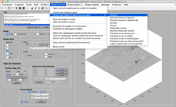
Coordinates of picked particles are represented by data types called models. In the tomoslicer window go to Model Pool -> Create new model in pool (choose type) -> General. This is the simplest type of model where each clicked/model point corresponds to a single isolated particle. Now you can navigate up and down the tomogram, center the mouse on the particle and click “C” to add a new model point. (Note the Help -> Shortcut options that lists the different the actions of the different keystrokes). Backspace button deletes the last clicked point.
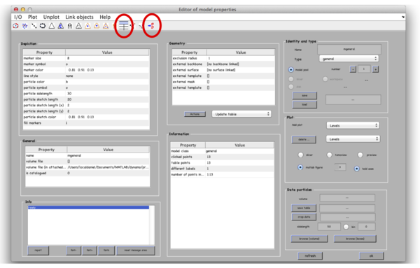
After you are done clicking a dozen of particles go to Active model -> Edit active model. This is a summary of the model with control elements for geometric transformations. Models of type general don’t allow any geometrical transforms, all you need to do here is to convert the clicked model points into “table points” that will be used for cropping. This is done by clicking the table-looking command icon (4th from the right in the top left part of the Editor of model parameters window). Alternatively, you could just click on Active model > Update Crop points in the tomoslice window. 

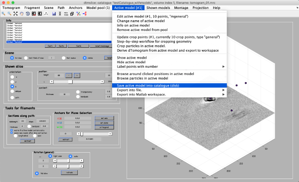
The model editor also gives you the possibility of changing the name of the model. You may want to give the models meaningful identifiers before storing them into disk. Also, you can open a GUI for extracting your particles (first icon from the right) to extract particles from only this tomogram, however we will do it later for all 3 tomograms. Make sure that the number of clicked points equals to the number of table points in the Information field and close the Editor window. Importantly, save the model into the catalogue by Active model -> Save active model into catalogue (disk) and close the slicer window. Pick particles for tomograms 2 and 3. In total, there are around 40 particles in the generated dataset.
 Important: when you open a new tomogram, make sure that you delete the pool of models from memory (model pool > clear current pool from memory). This will have no effect onto the models stored in disk, and it is necessary in order to ensure that you are not mixing models from different tomograms.
An alternate visualization: orthogonal projections
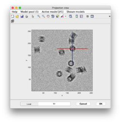
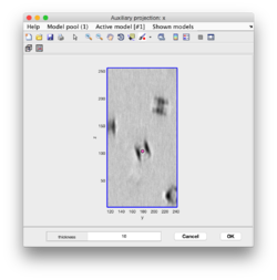
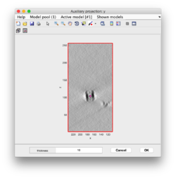
Clicking on Projection you will get a screen where the x-y projection of the tomogram is shown. Use the secondary click on it to launch the orthogonal views of x-z and y-z planes that traverse that point. Clicking on those views determines a 3D point.
Extracting particles from tomograms
In the catalogue manager window select the rows for tomograms from which you want to extract particles from. You can either select them one by one with a mouse click holding a CTRL button or click the “Select all” button. 

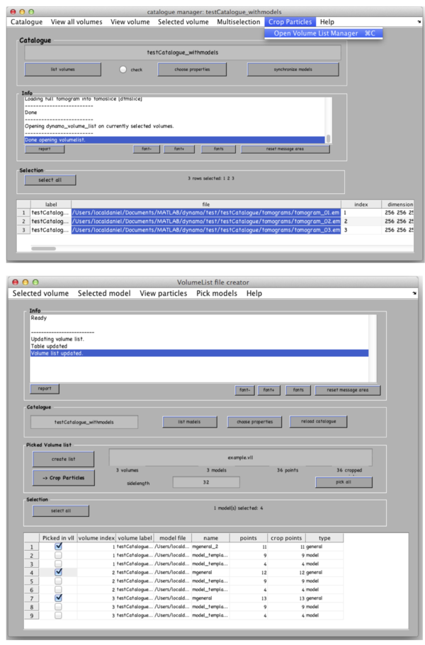
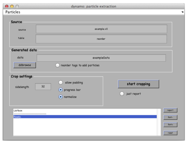
Go to Crop Particles -> Open Volume List Manager, all the models in the catalogue listed in the bottom of the window. Pick (by checking boxes) the models of type general – the ones that you have just clicked. Increase sidelength to 48-64 pixels. Vll-list is the format in which Dynamo stores directives for particle extraction; you can modify it with your own scripts if you have a lot of tomograms. Now click Create list and Crop particle. Change output directory name to i.e. “particles” and click “start cropping”.
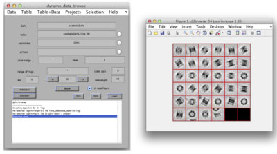
After cropping is done explore your cropped particles by clicking ddbrowse under the output folder name. ddbrowse (Dynamo Data Browse) is a lightweight browser for particle visualization, just click “show” and make sure your particles are well centered and fit the box. If not - use pre-existing models to generate the vll-file and re-extract the particles or increase the sidelength. Please note that Dynamo generated a particles/ folder with sub-volumes formatted as particle_000XX.em.

Subtomogram alignment and averaging
Initial model generation
If you don’t have an initial model it is easy to generate it by manually aligning several particles and summing them up. Dynamo stores information about the particles in dynamo tables: for each particle a table contains shifts and rotations to bring the particle to the average (by default these values are initialized as 0s), particle ID (tag), orientation of the missing wedge and others. For full info type >> dthelp in Matlab. Dynamo catalogue generates an initial table during particle extraction, its location is particles/crop.tbl
Loading particle in dgallery
For initial model generation we will use dynamo_gallery to generate initial orientations for some of our particles. Type
>> dgallery(‘data’, ‘exampleData.Data’);
assuming you named exampleData your data folder while cropping.
- Load particles into memory by clicking “load” in the Load from disk field on the left of the window. Note that at first, the scene will show only one particle.
- Display some or all of the particles with the slider in the Shown particles field on the top of the window.
- Toggle between X- Y- and Z-views in the View: orientation field.
Manual alignment of particles in dgallery
Now for each particle you can specify the center with a mouse click and the “C” button. Thermosomes are barrel-like particles with a long axis, you therefore may also specify the “top” of the particle by clicking along the long axis of the particle (but still within the box) with a mouse click and click “N” (stands for North). Do it for all the particles alternating the X- Y- and Z- views. Non-aligned particles are marked red, once the particle has been left-clicked it adds to the section in memory and turns blue. To remove from selection right click on the box.
Selecting particles in dgallery
You can save selected tags and a corresponding dynamo table by clicking the “quick save” button in the Particle Section field on top of the window. It saves a quickbuffer.tbl and quickbuffer.tags to the hard drive that you will use later.
Averaging selected particles
To generate the average you need to “apply” the table on the particles. For this click the “average” button in the Particle selection field. It opens dynamo_average_GUI with a lot of controls, we only need output filename in the Averaged volume field - my_average.em. Click “compute average” in the bottom of the window; wait till it is done. Right click to the output filename and select the [view] simple 3d depiction of all slices option and examine it from X- Y- and Z- views. If you are not satisfied with the result close the window and refine your manual alignment / add more particles to the average.
Alignment projects
Iterative alignment of subtomograms to the average is performed by dynamo projects that you can run in various high-performance computational environments. To have a project you need particles, an initial reference and a table which you have already generated. Start a WIZARD in the Dynamo command window or type
>> dcp
in Matlab (dcp stands for dynamo current project). Type a project name “drun1” and press Enter, Dynamo will generate the auxiliary files in a folder called drun1.
Linked files
Provide input in the popup windows: folder with particles (and press OK), initial table particles/crop.tbl. You can also provide the quickbuffer.tbl which has the initial orientations from manual picking, however remember that this table contains only the selected particles. In cases when you don’t have a table you can generate a blank or a random tables that would be consistent with your particle folder but will lack the metadata i.e. real missing wedge values or source tomograms. Go to “template” and input my_average.em. Go to “Masks”, here you can provide several masks for different purposes, now we are only interested in the alignment mask. Use ellipsoid, you can specify semi-axis or go to “Mask editor” to make more sophisticated masks. Note that Dynamo by default uses Rossman correlation which eliminates the artefacts associated with hard (non-soft) mask. As usual you right click on the mask that you generate in order to open it with dview. For this type of simulated data “use default masks” will work.
Numerical parameters
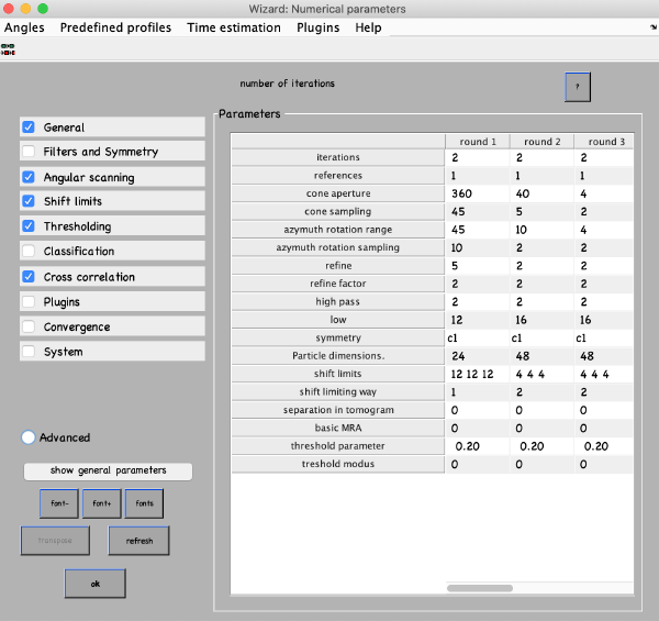
Numerical parameters menu provides flexibility on how to run your alignment. You can specify different parameters for different rounds of refinement. You can select any value in the table with a mouse and click the “?” button on the top right of the parameter window, this will give you more info. For more parameters check boxes on the left. The most important parameters to consider are:
- Number of iterations in each round. Make 2 rounds with 3-4 iterations in each. The first round will be global search with a course angular step, the second – constrained search with a finer step. If you decided to use a table with prealigned particles (quickbuffer.tbl) you may skip the first round.
- Angular search ranges: cone aperture is the scan range for the first two Euler angles with a step of cone sampling starting at the actual angles stored in the table. 360 is the full scan range. Azimuth rotation range defines rotation range around the new vertical axis of the particle
- High- and lowpass values in Fourier voxels limit the used frequency range. It can be autotuned (below in this manual), here use some reasonable values like half-Nyquist.
- Particle dimensions – use the sidelength of your box; if you put lower value the particles will be downsampled for the particular round. This will speed up the process.
- Refine after each angular scan the search step reduces refine factor times, this repeats refine times. I.e. if your cone sampling is 10 deg, refine and refine factor and 3 and 2 then 10, 5, 2.5 and 1.25 degrees will be sampled. This is the optimization of angular search space. We typically use 2 and 2.
- Shift limits limits translation of particles from the center of the box (if shifts limiting way is 1) or from the previously estimated center (if shifts limiting way is 2). The previous estimates for the shifts and rotations are taken from input tables and are updated at the end of each iteration.
- Symmetry – if you know the symmetry of your protein it will speed up the convergence and result in higher resolution. Here we don’t make any assumptions.
- Threshold parameters and modus specify which particles contribute to the average at the end of each iteration. Our typical values are [1,2] and [0.5,5].
There are predefined parameter sets for Global and Local searches (Predefined profiles -> Global search / Refinement). After you set up the parameters press OK or close the window. 
Go to Computing environment in Wizard and select Matlab-CPU. Click “Info (nvidia)” it should output you a table to your Matlab window, your GPU identifiers are in the left column of the table. Put those into the GPU identifiers to the ‘identifiers” field.
Running the project
Go back to the Wizard window, click “check” and ‘unfold”, this will generate a runnable matlab script drun1.m. If you will modify your project and will want to run it again you need to re-unfold the project before each run.
- In a Matlab session you can just click on “run”.
- In a standalone project it's more convenient to open a new terminal, activate Dynamo on it and run the project just invoking the name of the project script that was generated by the unfolding step:
./drun1.exe
Open another Matlab window, activate dynamo, go to the same folder and monitor the progress of the execution by typing in >> dvstatus drun1. After several iterations you can look at intermediate results by typing:
>> ddb drun1:a –v
or
>>ddb drun1:a:ite=* -j c10
For more info on ddb type >> help ddb. In the end of your iterations you can monitor the results in the show results section of Wizard and should get something like this:

Subtomogram classification
First generate a dataset which has 2 populations of particles. For this, type:
>> dynamo_tutorial('data_classification','M',8,'N',8);
in your Matlab window. It generates two sets of particles, 8 particles in each and stores their real orientations in the directory data_classification.
Multireference alignment
The idea behind MRA is: iterative alignment of particles to several references and then each particle assigned to the reference where it fits the best. This way over iterative refinement similar particles will have higher correlation to similar references and will eventually group together. MRA is naturally implemented in Dynamo. For classification into N classes we will need N initial references and N initially identical tables that Dynamo will generate automatically. The references should be slightly different to start particle differentiation, in Dynamo we add a small amount of white noise to the overall average of all particles.
Creating MRA projects
Create a new project by typing “drun2” in the project name of Wizard set number of references to 2, set Swap particles on, put in the particle data.
Seeds for MRA projects
- Go to “table” and type data_classification/real.tbl into the “clone this” field and press “copy”, press “OK”.
- Go to “template” and clone data_classification/original_template.em with addition of some extra noise with amplitude 1.
- Initialize masks with the defaults parameters (large button on the bottom).
Go to “numerical parameters” and use Predefined profiles -> refinement. Increase angular search steps to 5, set a thresholing policy and press “OK”. Set computing environment to GPU (under Matlab), specify GPU identifiers.
Execution of projects
Check, unfold and run the project, this project will run twice longer as each particle will be aligned to two references. Monitor the progress of your project by
>> dvstatus drun2
and visualize the results as
>> ddb drun2:a:ref=* -j c5
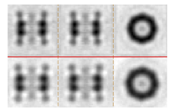
You should get something like this – two averages with particle in one class larger than in the other.
Classification with PCA and k-means
An analytical method is described in a tutorial classification_tutorial.pdf, please refer to it with dhelp.
Adaptive bandpass filtering
Aligning all particles to one reference may introduce overfitting resulting in resolution overestimation and a risk of overinterpretation of the final map. This is illustrated by a small exercise in the noise_artifacts.pdf tutorial. For the generation of the final map it is therefore highly recommended to separate your particles into two halves and perform independent alignment and averaging, using an Adaptive bandpass filtering approach: at the end of each iteration you can detect the current resolution by Fourier Shell Correlation and only use your reliable frequencies for the alignment at the next steps.
To perform independent half-dataset refinement load your initial project drun1 to Wizard (type in the Project field and press Enter or use Ctrl+L). Go to Multireference -> Adaptive filtering -> Derive a project, Dynamo will generate a new project drun1_eo, load it, inspect/update the parameters and run it. After it is done you can measure your resolution based on fsc plots from Multireference -> Adaptive filtering -> Plot attained resolution and inspect the average the usual way. 
