Starters guide (Copenhagen 2024)

This tutorial shows how to manually pick particles in a tomogram, extract them, align and classify them. This tutorial is a shortened version of the original starters guide that was adapted for the use in Dynamo workshops.

Manual particle picking and Dynamo catalogues

The Dynamo catalogues are databases that manage tomograms and link the tomographic data to the extracted particles. Start the catalogue manager by typing the command:

dcm

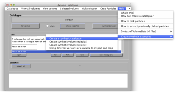
After the catalogue manager opens, we create 3 synthetic tomograms that include our particles (thermosomes) in the following way:

Figure 1: creating a set of synthetic tomograms with Dynamo Catalogue Manager

You can see the list of your tomograms and their metadata in a table in the bottom of your catalogue manager. When workin on your own projects, you can add tomograms to the catalogue by Catalogue -> Browse for new volume. The tomograms are situated in the directory testCatalogue. They contain a small amount of noise and a missing wedge associated to rotation around Y-axis. We added the information about location of the particles in the tomograms in an additional catalogue called testCatalogue_withmodels. If needed, it can be opened from the current folder with Catalogue -> look for local catalogues in the catalogue manager window.

Viewing tomograms

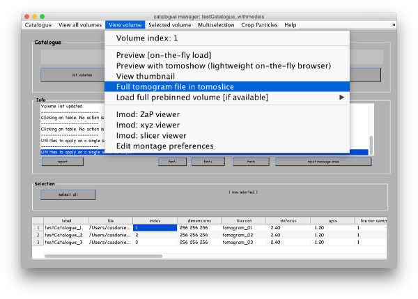
Select the first tomogram in the list and go to View volume>Full tomogram file in tomoslice.

Figure 2: Selecting a volume in the catalogue manager to be inspected in dpreview

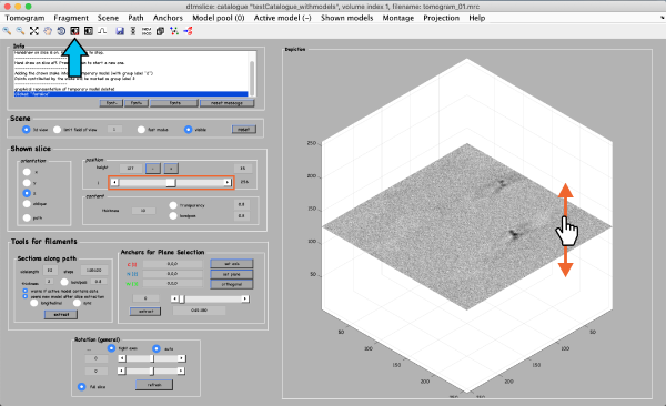
The volume browser tomoslicer loads the entire tomograms into memory and allows making annotations to the regions of interest. The tomograms in this tutorial are small, and you can load them directly into memory. For real life tomograms, bear in mind that you will need to prebin the files before loading them into memory. Tomoslice has a simple set of controls and is suitable for visualization tasks that require oblique sections through the tomogram. It uses the same tool as other Dynamo browsers to keep track of your annotations: a pool of models. You might need to adjust the contrast (blue arrow). To move through the tomogram slices, you can either use the mouse wheel, click and drag the tomogram slice up and down (orange arrows), or move the position control left and right (orange box).

Picking and extracting particles in tomograms

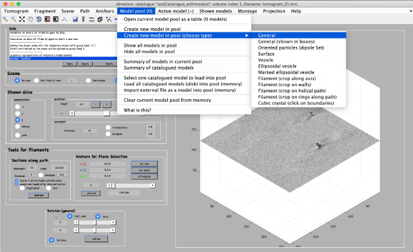
Coordinates of picked particles are represented by data types called models. In the tomoslicer window go to Model Pool -> Create new model in pool (choose type) -> General. This is the simplest type of model where each clicked/model point corresponds to a single isolated particle. Now you can navigate up and down the tomogram, place the mouse on the center of a particle and press the [c] key on your keyboard to add a new model point. (Note the Help -> all hot keys options that lists the different the actions of the different keystrokes). Backspace button deletes the last clicked point (you can also use the right-click to delete single points).

Generating a new model

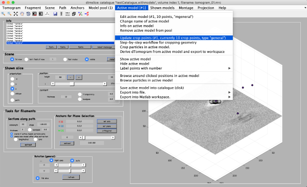
After you are done clicking about 10 particles click on Active model > Update Crop points in the tomoslice window. 

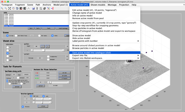
Save the model into the catalogue by Active model -> Save active model into catalogue (disk) and close the slicer window.

Pick particles for tomograms 2 and 3. In total, there are around 30-40 particles in the generated dataset. When you open a new tomogram, make sure that you delete the pool of models from memory when asked. This will have no effect onto the models stored in disk, and it is necessary in order to ensure that you are not mixing models from different tomograms.

An alternate visualization: orthogonal projections

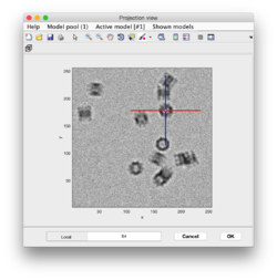
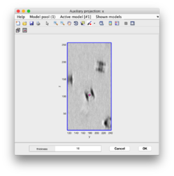
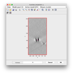
Clicking in the menu on Projection -> project full shown fragment along z (still in dtmslice) and you will get a screen where the x-y projection of the tomogram is shown. Use the secondary click on it to launch the orthogonal views of x-z and y-z planes that traverse that point. These views can also be used to click particles, in case the standard view is not sufficient.

click on the main projection determines two orthogonal slices

Slice xz

Slice xy

Extracting particles from tomograms

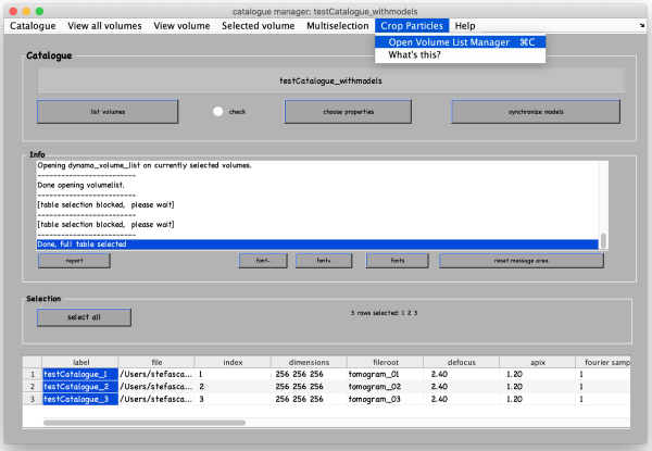
In the catalogue manager window select the rows for tomograms from which you want to extract particles from. You can either select them one by one with a mouse click and holding the [ctrl] key or by clicking the Select all button. Then, go to Crop Particles -> Open Volume List Manager.

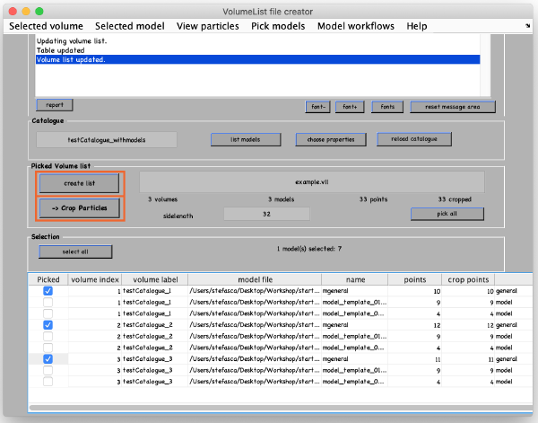
A new window opens with all the models in the catalogue listed in the bottom. Pick (by checking boxes) the models of type general that you have just clicked. Click Create list and then Crop particle.

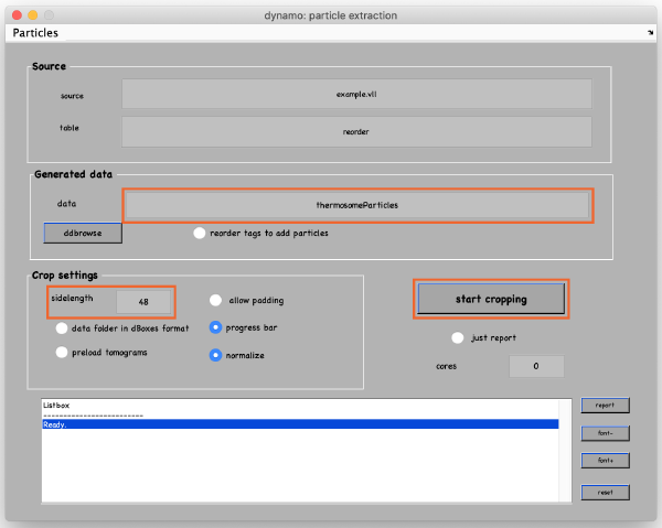
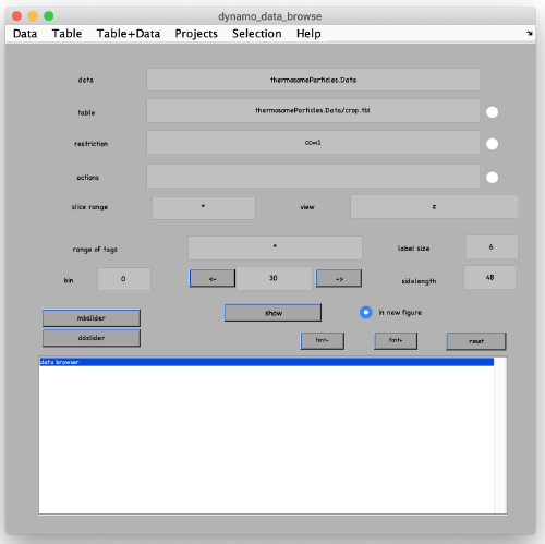
In the new window, change the data name to something meaningful, such as thermosomeParticles, change the sidelength from 32 to 48 and click start cropping.

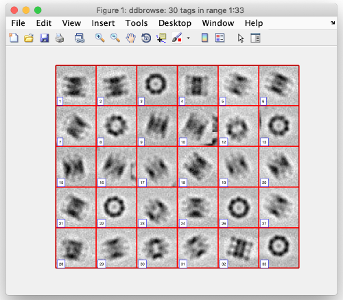
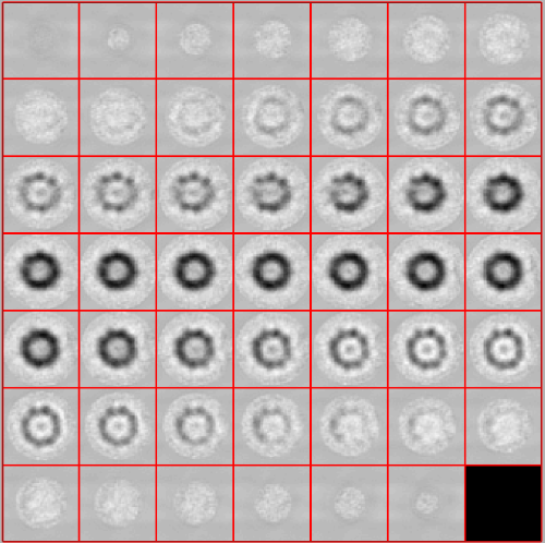
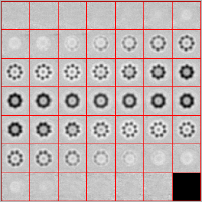
After cropping is done, explore your cropped particles by clicking ddbrowse (in the window above). A new window opens where you can simply click on show.

You see a 2D representation (projections) of all cropped 3D subtomograms. Make sure your particles are well centered and fit the box.

We also introduce the concept of the dynamo table: The information about each particle is stored in tables. Each particle has an entry in the table that contains shifts and rotations to describe its orientation (by default these values are initialized as zeroes). It also contains the particle ID (tag), the orientation of the missing wedge and others. For full info type the command dthelp. The Dynamo catalogue generates an initial table during particle extraction. Its location is in particles/crop.tbl .

Subtomogram alignment and averaging

Initial reference generation

We want to align the extracted tomograms to a common reference. For that, we need an initial reference (which will later be refined during the iterative alignment). Here, we create such an initial reference by manually align a few particles and average them. We use the command dgallery to generate initial orientations for some of our particles that will be used to generate the initial reference. Close all open Dynamo windows and type into the Dynamo command line:

dgallery('data','thermosomeParticles.Data');

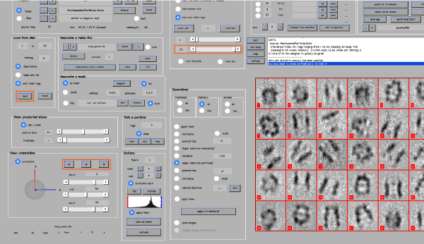
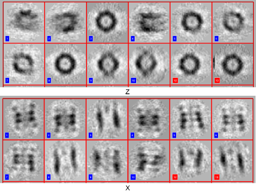
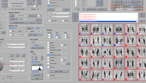
The gallery opens. Click on load to load all aprticles in memory, move the shown bar to display the particles and use the x-, y- and z-buttons to see different views:

To manually align the particles, do the following for about 10 particles:

1. Place the mouse over the particle center and press the key [c] (this centers the particle).
2. Place the mouse over its top (or bottom) part and press the key [n] (this aligns the particle).
3. Click on the particle to make sure its number turns from red to blue (blue means it is selected for further processing). To de-select a particle use the right-click.

Change between the x-, y- and z-views to correct the orientations if necessary. This is just done to create an initial reference, so orientations don't need to be very exact.

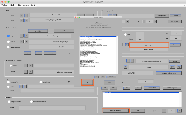
Save the selected tags and corresponding table by clicking quick save button in the top right. It saves a quickbuffer.tbl and quickbuffer.tags to the hard drive that will be used later. To generate the average you need to apply the table on the particles. For this click the average button in the Particle selection field.

It opens a new window with a lot of controls. Click compute average in the bottom of the window. Then, right-lick on the output filename and click ok in the next window to see the result. If you are not satisfied with the result, close the window and refine your manual alignment and/or add more particles to the average.

Alignment projects

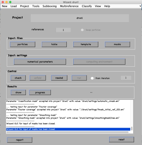
Iterative alignment of subtomograms to their average is performed by dynamo projects that you can run in various high-performance computational environments. To run an alignment project you need the particles, an initial reference and a table. All of these files we generated before. Start the alignment project GUI by typing

 dcp

In thw new window, do the following:

1. Add the project name drun1, press the enter key and select create a new project in the pop-up window.
2. Click on particles and provide the particle folder name thermosomeParticles.Data. Click ok.
3. Click on table and provide the table name thermosomeParticles.Data/crop.tbl. Click ok.
4. Click on template and provide the initial reference name my_average.em. Click ok.
5. Click on masks and simply click on use default masks. Click ok. You could also specify the semi-axis of the ellipsoid masks or go to “Mask editor” to make more sophisticated masks. Note that Dynamo by default uses Rossman correlation which eliminates the artefacts associated with hard (non-soft) mask.

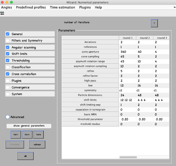
Click on numerical parameters to set all parameters and details about the different iterations of the alignment project. You can select any parameter in the table with a mouse and click the ? button on the top right of the parameter window to see a description of the parameters. The most important parameters to consider are:

• Number of iterations: Make 3 rounds with 2 iterations each. The first round will be a global search with a coarse angular step and the following rounds will be used for refinement.
• Angular search ranges: Cone aperture is the scan range for the first two Euler angles around the initial orientation defined in the table. 360 degrees is the full scan range. Azimuth rotation range defines the rotation range around the new vertical axis of the particle.
• High- and lowpass values: Fourier voxels to limit the used frequency range.
• Particle dimensions: Defined as sidelength of your subvolume. If you put a lower value, the particles will be downsampled for the particular round. This will speed up the process.
• Refine: After each angular scan, the search step is reduced by the refine factor. This is repeated refine times. I.e., if your cone sampling is 10 degrees, refine is 3 and refine factor is 2, then 10, 5, 2.5 and 1.25 degrees will be sampled. This is the optimization of angular search space.
• Shift limits: Limits the translation of particles from the center of the box (if shifts limiting way is 1) or from the previously estimated center (if shifts limiting way is 2). The previous estimates for the shifts and rotations are taken from input tables and are updated at the end of each iteration.
• Symmetry: If you know the symmetry of your protein it will speed up the convergence and result in higher resolution.

Set the parameters as follows and click ok:

Click on Computing environment and select your computing environment (choose standalone if you are working on the standalone version during a workshop). Set CPU cores and parallelize averaging step to the maximum available (e.g., 4). Leave the rest as it is and click ok. In the alignment GUI click check and unfold. To run the project

• in a Matlab session, you can just click on “run”.
• in a standalone project it is more convenient to open a new terminal, load Dynamo (but do not run it) and run the project by typing ./drun1.exe.

While the project is running, open another Matlab window (or in standalone open another terminal with Dynamo running) and you can monitor the progress of the alignment project by typing:

dvstatus drun1

While the project is running, you can look at projections of the intermediate results by typing:

ddb drun1:a:ite=* -j c10

or at the latest average by typing:

ddb drun1:a -v 

The final result should look similar to:

Results of alignment.



Subtomogram classification

To demonstrate a classification example we provide particles with 2 slightly different sizes. We can then classify them with a simple Multi-reference Analysis (MRA). To do that, we first generate a dataset which has 2 populations of particles. For this, type:

dynamo_tutorial('data_classification','M',8,'N',8);

It generates two sets of particles, 8 particles in each including their table. The idea behind MRA is the following: The particles are aligned to several references (here only 2). After each iteration, each particle is assigned to only one single reference where it fits the best. This procedure is repeated iteratively. Similar particles will have higher correlation to similar references and will eventually group together. For classification into N classes we will need N initial references and N initially identical tables.Follow these steps to run the MRA:

1. Create a new project by typing “drun2” in the project name of the alignment GUI.
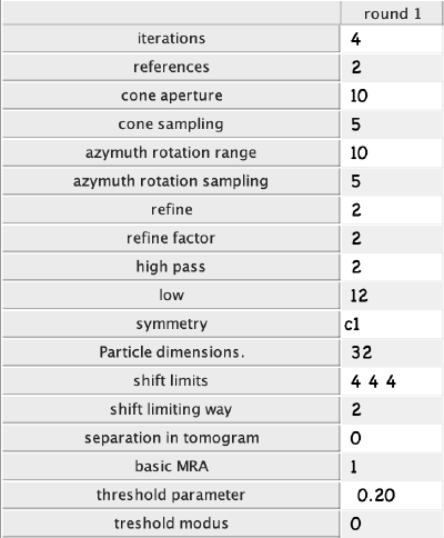
2. Set number of references to 2.
3. Activate the Swap particles button.
4. Go to particles and add data_classification/data to the particle data. Click ok.
5. Go to table and type data_classification/real.tbl into the field clone this and press copy. Click ok.
6. Go to template and clone data_classification/original_template.em with addition of some extra noise with amplitude 1.
7. Click on masks and click on use default masks. Click ok.
8. Click on numerical parameters and set the following parameters. Click ok.

Choose the same computing environment as in the previous alignment project and run the project in the same way too. MRA projects usually run longer, because each particle will be aligned to two references. Here, however, we chose the parameters in a way that the process is still fast (e.g., small dimensions). Monitor the progress of the project same as before:

dvstatus drun2

And visualize the results using the command:

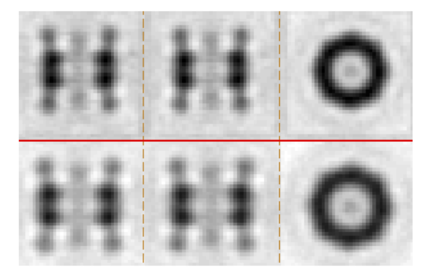
ddb drun2:a:ref=* -j c5

You should get two averages with particle in one slightly class larger than in the other.

Results of classification.